The Returns to Neighborhood Quality Depend on Who You Are
Shrey Shah
This paper is part of a collection of unpublished economics papers.
The additive model of neighborhood effects assigns the wrong sign to the amenity interaction for families below the 34th percentile of the income distribution—the families housing policy primarily targets. Using the Opportunity Atlas, we estimate the interaction between school quality and neighborhood wealth at six parental income percentiles within the same census tract. The interaction declines monotonically from +0.003 at $p1$ (complements) to -0.007 at $p100$ (substitutes), crossing zero at the 34th percentile ($t = 26.1$; $N = 142{,}068$). A model of private substitution generates this gradient as an equilibrium prediction. A school boundary regression discontinuity ($\tau = 0.025$, $p < 0.001$) and cross-race tests ($t = 3.24$) provide supporting evidence. The gradient is steeper for Black and Hispanic children, consistent with greater barriers to private substitution. All six percentile-specific coefficients survive Bonferroni correction; the gradient replicates across genders and within race groups.
1. Introduction
Where should a low-income family live to maximize their children’s long-run outcomes? The standard approach assigns each neighborhood an “opportunity score” that adds up amenity levels. This additive model gets the direction of the amenity interaction wrong for families below the 34th percentile of the income distribution—the families that housing vouchers and place-based policies primarily serve.
Neighborhoods causally affect intergenerational mobility (Chetty and Hendren, 2018a; Chetty and Hendren, 2018b; Chetty and Friedman, 2018). Subsequent work has identified specific mechanisms—school quality (Black, 1999; Chetty and Friedman, 2011), neighborhood income composition (Ludwig et al., 2013; Chyn, 2018), and social capital (Chetty and Jackson, 2022a; Chetty and Jackson, 2022b)—but these have been studied in isolation. In reality, families choose a location that bundles all amenities together. Whether these amenities are complements or substitutes has remained an open question.
Using the Opportunity Atlas, which reports outcomes at every parental income percentile within the same census tract, we estimate the interaction between school quality (SQ) and neighborhood wealth (W) at six percentiles from $p1$ to $p100$. Because all tract-level amenities are identical across percentiles, variation in the interaction reflects differential sensitivity to local amenities rather than sorting on amenity levels. The W $\times$ SQ interaction declines monotonically from $+0.003$ at $p1$ to $-0.007$ at $p100$, crossing zero at the 34th percentile (Figure 1). For low-income families, amenities are complements: the effect of a good school is amplified by wealthy neighbors. For high-income families, amenities are substitutes: one can compensate for deficiencies in the other.
A model of private substitution generates this gradient as an equilibrium prediction. Families invest in private alternatives at a rate increasing in income and decreasing in local amenity quality, yielding an interaction coefficient $\gamma(p) = 1 - \phi\kappa p(\delta - \phi Q)$ that declines linearly in parental income. The model predicts that the sign reversal should be specific to outcomes amenable to private substitution and absent for outcomes determined by the local environment regardless of family resources.
Supporting evidence comes from two additional designs. A school attendance boundary regression discontinuity across five states yields $\tau = 0.025$ ($p < 0.001$), confirming that school quality affects mobility. Cross-race tests show the gradient is steeper for Black and Hispanic children ($t = 3.24$), consistent with greater barriers to private substitution among minority families. The gradient replicates across genders, with all six percentile-specific coefficients surviving Bonferroni correction.
The additive model that has dominated the literature is a reasonable approximation for middle-income families but gets the direction wrong for the poorest and richest.
The remainder of the paper proceeds as follows. Section 2 presents the model. Section 3 describes our data. Section 4 details the empirical strategy. Section 5 presents results: the cross-percentile gradient, corroborating designs, and robustness. Section 6 concludes.
2. Model
2.1 Setup
A child $i$ grows up in tract $\ell$ with school quality $S_\ell$ and neighborhood wealth $W_\ell$. The family has permanent income at percentile $p_i \in [0,1]$ of the national distribution. The child’s long-run outcome (income rank at age 35) is determined by a production function over local amenities and private parental investment.
2.2 Production Function
The child’s outcome depends on two inputs: the local amenity bundle $Q_\ell = S_\ell \cdot W_\ell$ and private investment $I_i \geq 0$ (tutoring, enrichment, private schooling, professional networks): \(Y_i = \underbrace{\beta_S S_\ell + \beta_W W_\ell}_{\text{additive amenity effects}} + \underbrace{Q_\ell \cdot (1 - \phi I_i)}_{\text{interaction, moderated by investment}} + \underbrace{\delta I_i}_{\text{direct investment effect}} + \varepsilon_i\)
where $\phi > 0$ governs the rate at which private investment substitutes for local amenity complementarity: when $I_i$ is high, the interaction $Q_\ell$ matters less, because the family has privately replaced what the neighborhood would otherwise provide.
The cross-partial derivative of outcomes with respect to $S$ and $W$ is: \(\frac{\partial^2 Y_i}{\partial S \, \partial W} = 1 - \phi \, I_i^\ast\)
This is the key object: the effective complementarity of local amenities depends on how much the family invests privately.
2.3 Optimal Private Investment
Families choose $I$ to maximize child outcomes net of cost. The cost of investment is $c(I; p) = \frac{I^2}{2\kappa p}$, where $\kappa > 0$ and higher-income families face lower marginal costs (reflecting both budget constraints and access to educational markets). The family solves: \(\max_{I \geq 0} \;\; \delta I - \phi Q_\ell \, I - \frac{I^2}{2\kappa p}\) The first-order condition gives optimal investment: \(I^\ast(p, Q_\ell) = \kappa p \, (\delta - \phi Q_\ell)\)
provided $\delta > \phi Q_\ell$ (the direct return to investment exceeds the substitution cost). Investment is increasing in family income $p$ and decreasing in local amenity quality $Q_\ell$—richer families invest more, and families in better neighborhoods invest less, because private investment and local quality are substitutes.
2.4 The Cross-Percentile Gradient
Substituting optimal investment (Eq. 4) into the cross-partial (Eq. 2): \(\gamma(p) \equiv \frac{\partial^2 Y}{\partial S \, \partial W}\bigg|_{I=I^\ast} = 1 - \phi \kappa p \, (\delta - \phi Q_\ell)\)
Holding $Q_\ell$ fixed (as in our within-tract design): \(\frac{d\gamma}{dp} = -\phi \kappa (\delta - \phi Q_\ell) < 0\)
This is the central prediction: the effective complementarity of local amenities declines monotonically in family income. The gradient is steeper when private investment is cheap ($\kappa$ large) and when the substitution rate ($\phi$) is high.
Proposition 1 (Cross-Percentile Gradient). Under the production function (Eq. 1) with optimal investment, the $S \times W$ interaction coefficient $\gamma(p)$ is:
-
Positive (complements) for $p < p^\ast$ and negative (substitutes) for $p > p^\ast$, where $p^\ast = \frac{1}{\phi\kappa(\delta - \phi Q_\ell)}$
-
Monotonically declining in parental income percentile $p$
-
Linear in $p$, with slope $-\phi\kappa(\delta - \phi Q_\ell)$
The linearity prediction is directly testable: plotting $\hat{\gamma}_p$ against $p$ should yield an approximately linear, downward-sloping relationship.
Calibration.
We observe $\hat{\gamma}_p$ at six percentiles ($p \in {1, 10, 25, 50, 75, 100}$). The linear model $\gamma(p) = a - bp$ identifies the composite parameter $b = \phi\kappa(\delta - \phi\bar{Q})$ and the crossover point $p^\ast = a/b$. In Section 5, we estimate $p^\ast \approx 34$, implying that amenities are complements for roughly the bottom third of the income distribution and substitutes for the top two-thirds. For the families that housing policy targets (below the median), complementarity is the dominant regime.
Welfare implications.
The model provides a welfare metric for housing placement. For a family at percentile $p$ placed in tract $\ell$, the complementarity premium is $\gamma(p) \cdot S_\ell W_\ell$. Summing over families placed by a housing program, the aggregate welfare gain from complementarity-aware siting relative to additive siting is: \(\Delta \mathcal{W} = \sum_{i} \gamma(p_i) \cdot S_{\ell_i^{\text{int}}} W_{\ell_i^{\text{int}}} - \gamma(p_i) \cdot S_{\ell_i^{\text{add}}} W_{\ell_i^{\text{add}}}\)
where $\ell^{\text{int}}$ and $\ell^{\text{add}}$ are the interaction-optimal and additive-optimal tract assignments. This welfare gain is largest for low-$p$ families (where $\gamma(p)$ is most positive) placed in high-$Q$ tracts.
2.5 Additional Predictions
In the empirical analysis, we implement the gradient test using: \(Y_{tp} = \alpha_t + \gamma_p \cdot (W_t \cdot S_t) + \beta_p \cdot W_t + \mu_p \cdot S_t + \varepsilon_{tp}\)
where $t$ indexes tracts and $p$ indexes parental income percentile. The tract fixed effect $\alpha_t$ absorbs all time-invariant tract characteristics, and identification of $\gamma_p$ comes from within-tract, across-percentile variation. The model generates two additional predictions:
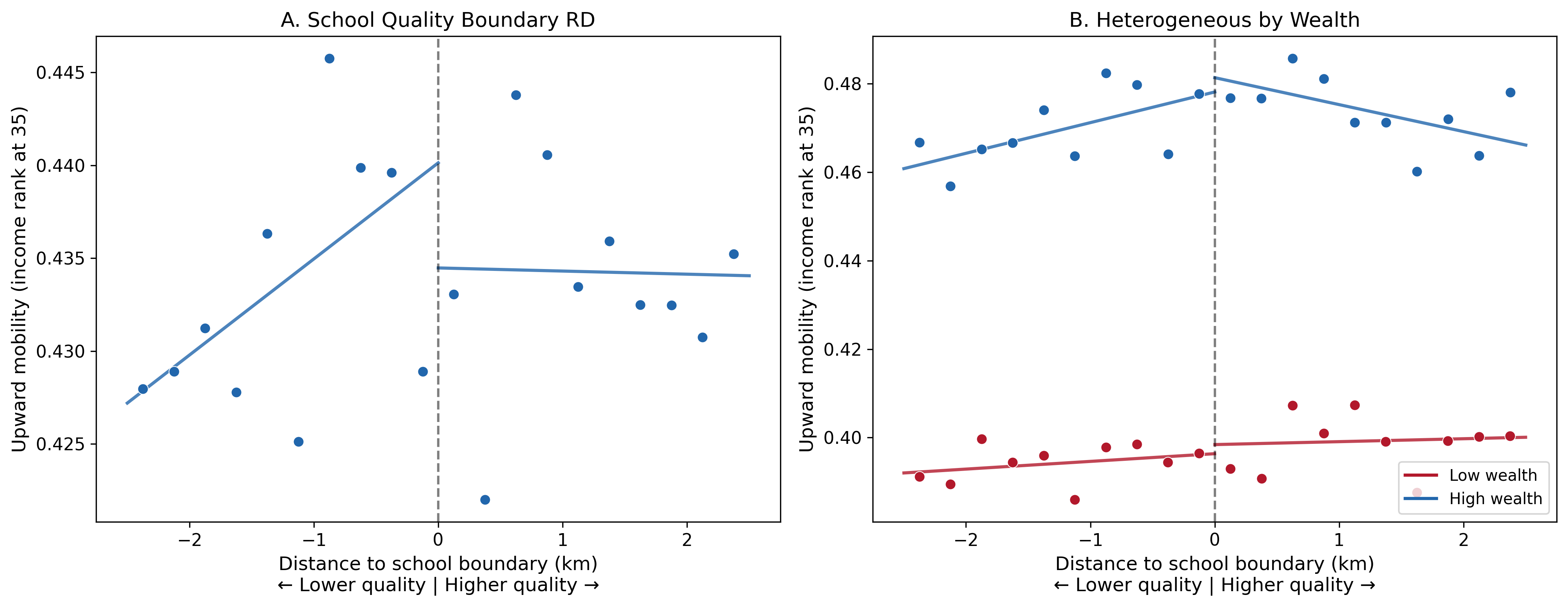
Proposition 2 (Heterogeneous School RD Effects). If $S$ and $W$ are complements ($\gamma_{SW} > 0$), the school attendance boundary RD effect on mobility should be larger in wealthier neighborhoods.
Proposition 3 (Cross-Race Heterogeneity). If complementarity reflects differential access to private substitutes (and minority families face greater barriers to substitution due to discrimination, wealth gaps, and network exclusion), the gradient should be steeper for Black and Hispanic children than for white children.
3. Data
3.1 Outcomes and Cross-Percentile Structure
Our outcome data come from the Opportunity Atlas (Chetty and Friedman, 2018), which provides tract-level estimates of children’s mean household income rank at age 35, constructed from de-identified federal tax records for children born 1978–1983. The Atlas reports outcomes at every parental income percentile ($p1$ through $p100$) for pooled and race-specific (white, Black, Hispanic) subgroups.
Our primary outcome is mobility at $p25$ (the standard measure), but the cross-percentile structure is essential to our identification strategy. By stacking outcomes at different percentiles within the same tract, we hold all tract-level amenities constant and identify how the amenity interaction varies with family income. The data cover 71,034 tracts with non-missing outcomes at both $p25$ and $p75$.
3.2 Neighborhood Amenities
We measure three amenities at the tract level. School quality is constructed from standardized test scores linked to school attendance boundaries from the NCES School Attendance Boundary Survey (SABS), covering 75,128 attendance zones. We standardize within state. Neighborhood wealth is the first principal component of median household income, education share, poverty rate, and employment rate from the American Community Survey (ACS), standardized within commuting zone. Home values are excluded from the index to avoid endogeneity concerns. Economic connectedness (EC) is the cross-class friendship index from Chetty Jackson (2022a), matched to 58,804 tracts via the Census 2020 ZCTA-tract crosswalk.
The correlation between school quality and wealth is moderate (0.47), while EC is nearly orthogonal to both ($-0.08$ and $0.06$), indicating genuinely distinct dimensions of neighborhood quality.
3.3 School Boundary Pair Data
For the RD analysis, we process five states (TX, FL, IL, OH, PA) using SABS attendance zone boundaries, identifying 86,102 adjacent zone pairs sharing at least 50m of boundary (691,158 observations). We use the rdrobust package (Calonico et al., 2014; Calonico et al., 2020) for MSE-optimal bandwidth selection and bias-corrected inference.
3.4 Sample
The following table presents summary statistics.
Panel A: Outcomes
| Variable | Mean | Std Dev | 10th Pctile | 90th Pctile |
|---|---|---|---|---|
| Upward mobility (income rank at 35, $p25$) | 0.429 | 0.071 | 0.339 | 0.522 |
Panel B: Neighborhood Amenities
| Variable | Mean | Std Dev | 10th Pctile | 90th Pctile |
|---|---|---|---|---|
| School quality index | 0.000 | 1.000 | −1.266 | 1.263 |
| Neighborhood wealth index | 0.000 | 1.000 | −1.316 | 1.291 |
| Economic connectedness | 0.000 | 1.000 | −1.399 | 1.277 |
Table 1: Summary Statistics
Notes: Sample includes 72,793 census tracts. Upward mobility ($N = 71{,}538$) is the mean household income rank at age 35 for children with parents at the 25th percentile. All amenity indices standardized within state (SQ) or commuting zone (W, EC).
4. Empirical Strategy
We use three identification strategies. The first exploits the cross-percentile structure of the Opportunity Atlas and forms our primary test. The second and third provide supporting evidence from different sources of variation.
4.1 Primary: Cross-Percentile Gradient
The Opportunity Atlas reports outcomes at every parental income percentile within the same tract. Because all tract-level amenities are identical across percentiles, within-tract variation in the W $\times$ SQ interaction identifies differential sensitivity to complementarity, free of sorting.
We estimate the interaction at each of six available percentiles ($p1$, $p10$, $p25$, $p50$, $p75$, $p100$) using CZ-fixed-effects regressions: \(Y_{t,p} = \alpha_{cz} + \beta_W W_t + \beta_S S_t + \gamma_p (W_t \cdot S_t) + X_t'\theta + \varepsilon_t\)
where $\gamma_p$ is the W $\times$ SQ interaction at parental percentile $p$. CZ fixed effects absorb regional confounders; amenities are demeaned within CZ.
For the formal test, we stack $p25$ and $p75$ outcomes within each tract ($N = 142{,}068$) and include tract fixed effects:
\[Y_{tp} = \alpha_t + \delta_{p25} + \gamma \cdot (W_t \times S_t \times \mathbf{1}[p = 25]) + \beta_W (W_t \times \mathbf{1}[p = 25]) + \beta_S (S_t \times \mathbf{1}[p = 25]) + \varepsilon_{tp}\]The coefficient $\gamma$ tests whether the complementarity is stronger at $p25$ than $p75$. Tract fixed effects absorb all tract-level variation, so identification comes purely from within-tract, across-percentile differences.
4.2 Supporting: School Boundary RD
Following Black (1999), we exploit the sharp change in school quality at attendance zone boundaries. For each tract $t$ near boundary $b$: \(Y_t = \alpha_b + \tau \cdot D_t + \phi \cdot (D_t \times W_t) + \lambda W_t + f(d_t) + \varepsilon_t\)
where $D_t = \mathbf{1}[S_t > S_t^\ast]$ is the higher-quality-school indicator and $d_t$ is signed distance to the boundary. We use rdrobust for MSE-optimal bandwidth selection and bias-corrected confidence intervals for the basic RD ($\tau$). For the interaction ($\phi$), we use hand-coded WLS at the rdrobust-selected bandwidth, since the package does not natively support interactions.
4.3 Supporting: Cross-Race Test
Different racial groups in the same CZ face different effective amenity bundles. We stack race-specific outcomes and estimate: \(Y_{tr} = \alpha_{cz} + \beta_r \cdot \text{Race}_r + \phi_r \cdot (\text{Race}_r \times W_t \times S_t) + \varepsilon_{tr}\)
with CZ fixed effects absorbing all CZ-level confounders. The coefficient $\phi_r$ tests whether the W $\times$ SQ interaction differs by race.
5. Results
5.1 The Cross-Percentile Gradient
Figure 1 presents the main finding. Panel A plots the W $\times$ SQ interaction coefficient at each parental income percentile, estimated with CZ fixed effects on 71,034 tracts.
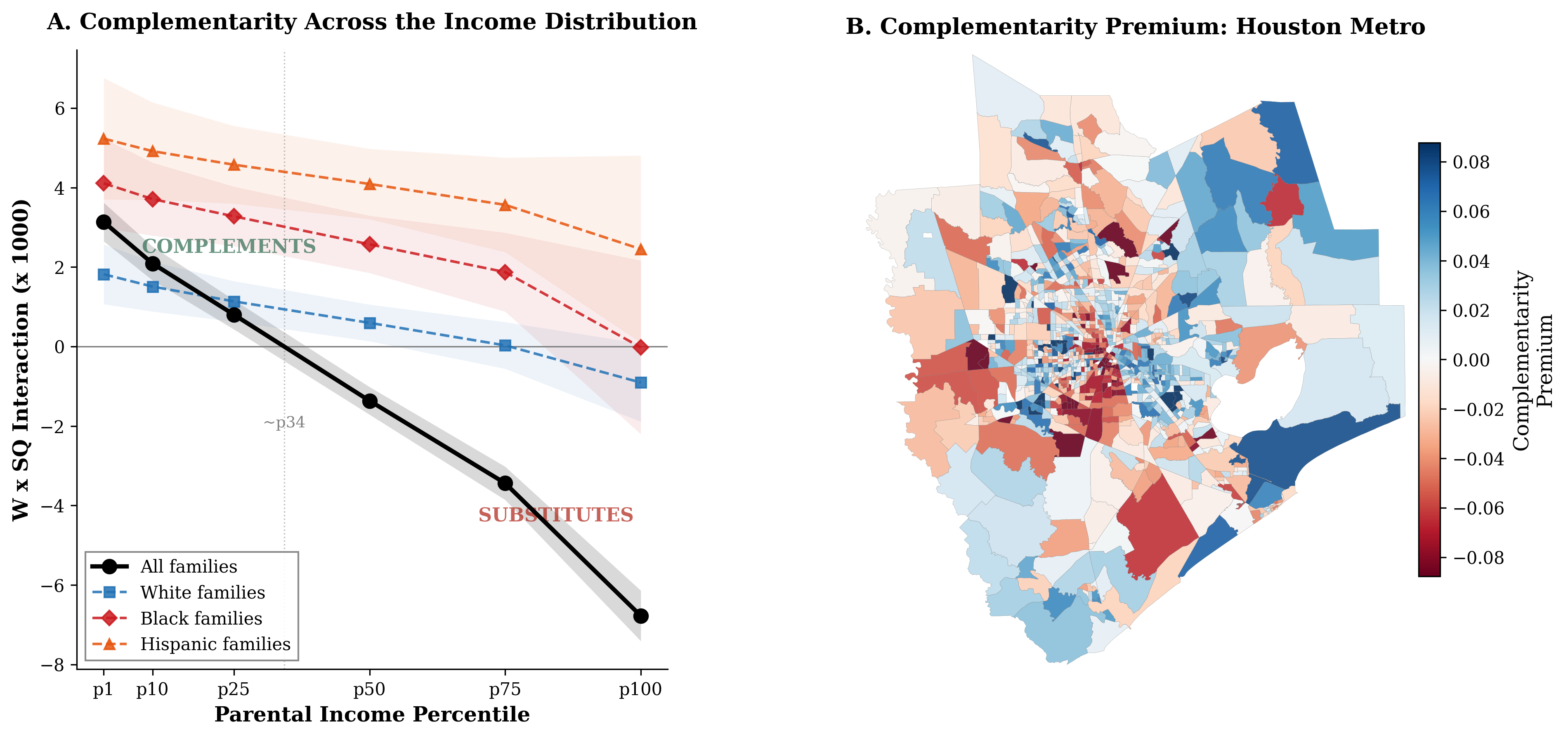
Notes: Panel A plots the W $\times$ SQ interaction coefficient from CZ-fixed-effects regressions at each parental income percentile. The thick black line shows pooled estimates; colored lines show race-specific gradients. Shaded bands are 95% confidence intervals. The gradient declines monotonically from complements (positive) for low-income families to substitutes (negative) for high-income families. Panel B shows the gradient by race. Black and Hispanic children exhibit complements at nearly every percentile, while White children cross zero near $p75$. $N = 71{,}034$ tracts.
The interaction is positive and significant at $p1$ ($+0.003$, $t = 4.8$ with CZ-clustered SEs) and $p10$ ($+0.002$, $t = 3.8$), weakly positive at $p25$ ($+0.001$, $t = 1.6$), and becomes negative at $p50$ ($-0.001$, $t = -2.0$), growing to $-0.003$ ($t = -3.5$) at $p75$ and $-0.007$ ($t = -4.4$) at $p100$. The gradient is monotonically declining across all six percentiles.
CZ-FE regressions by percentile ($N = 71{,}034$)
| W $\times$ SQ | SE(HC1) | $t$(HC1) | SE(CZ) | $t$(CZ) | $R^2$ | |
|---|---|---|---|---|---|---|
| $p1$ | +0.00313 | 0.00025 | 12.65 | 0.00066 | 4.77 | 0.346 |
| $p10$ | +0.00209 | 0.00022 | 9.63 | 0.00055 | 3.78 | 0.402 |
| $p25$ | +0.00080 | 0.00019 | 4.25 | 0.00051 | 1.58 | 0.466 |
| $p50$ | −0.00136 | 0.00018 | −7.68 | 0.00067 | −2.04 | 0.503 |
| $p75$ | −0.00344 | 0.00021 | −16.10 | 0.00097 | −3.54 | 0.413 |
| $p100$ | −0.00677 | 0.00032 | −20.92 | 0.00154 | −4.39 | 0.220 |
Table 2: The Cross-Percentile Gradient: W $\times$ SQ Across the Income Distribution
Notes: Each row reports the W $\times$ SQ interaction from a separate CZ-FE regression at the indicated percentile. HC1 and CZ-clustered ($N_{\text{CZ}} = 718$) standard errors reported.
Interpretation and magnitude.
For the poorest families ($p1$, $p25$), school quality and wealth are complements: neighborhoods that combine both produce outcomes exceeding the sum of parts. For the richest families ($p75$, $p100$), they are substitutes: high-income parents compensate for missing amenities, so the marginal effect of one is lower when the other is high. The crossover occurs at the 34th percentile.
The interaction adds only 0.1 percentage points to the within-CZ $R^2$ beyond main effects (Appendix Table 5). But the $R^2$ is the wrong test. The gradient reveals that the sign of the interaction reverses across the income distribution: from $+0.003$ at $p1$ to $-0.007$ at $p100$, a total range of 1.0 percentile rank or 7% of the $p10$–$p90$ mobility range. An additive model—regardless of its $R^2$—gets the direction wrong for the poorest and richest families: it understates complementarity by 0.3 percentile ranks at $p1$ and overstates it by 0.7 percentile ranks at $p100$. For a family at $p1$ moving from the interquartile range to the top quartile on both amenities, the complementarity premium is 0.6 percentile ranks; at $p100$, the substitution penalty is $-1.2$ percentile ranks. Across 9,402 tracts (13.2%), the complementarity premium exceeds 0.5 percentile ranks for $p1$ families. The interaction matters not because it adds explanatory power but because it changes who benefits.
This pattern is consistent with Proposition 1: low-income families rely on local amenities and benefit from complementary bundles; high-income families substitute privately and exhibit diminishing returns to the bundle.
Race-specific gradients.
Figure 1 (Panel B) shows the gradient by race. For Black children ($N = 33{,}883$ tracts), amenities are complements at every parental income level through $p75$ ($+0.002$, $t = 3.70$), crossing zero only at $p100$. For Hispanic children ($N = 37{,}217$), the interaction is positive at every percentile including $p100$ ($+0.002$, $t = 2.04$). For White children, the gradient is flatter, crossing zero near $p75$. These patterns are consistent with Proposition 3: groups that face greater barriers to private substitution remain amenity-dependent to higher income levels. Appendix Table 11 reports the full race-specific coefficients. The gradient replicates across genders, with the female gradient 45% steeper than the male gradient (Appendix Table 15).
Descriptive evidence.
Appendix Figure 6 shows $10 \times 10$ heatmaps of mobility by school quality and wealth decile at $p25$ and $p75$: the complementarity layer is visible in the raw data, concentrated in the upper-right corner (high SQ, high W). Appendix Figure 3 presents additional binned scatter plots by wealth quartile.
5.2 Corroborating Designs
School boundary RD.
Using rdrobust (Calonico et al., 2014; Calonico et al., 2020) with MSE-optimal bandwidth selection on 86,102 boundary pairs across five states, the school quality effect is $\tau = 0.025$ ($t = 20.1$, BW $= 0.121$ km, $N_{\text{eff}} = 9{,}915$): children on the higher-quality-school side of an attendance boundary have 2.5 percentile ranks higher mobility (Appendix Table 8, Appendix Figure 9). Balance tests show that wealth and demographic covariates also shift at the boundary (Appendix Table 6), so the RD identifies the joint effect of school quality and correlated neighborhood characteristics; we treat it as corroborating evidence. Spatial profiles show school quality jumps sharply while wealth varies more smoothly (Appendix Figure 5). Appendix Table 9 reports state-by-state estimates; Appendix Table 7 reports bandwidth sensitivity.
Cross-race evidence.
Stacking race-specific mobility within tracts (white, Black, Hispanic), the W $\times$ SQ interaction is positive and significant ($0.002$, $t = 3.24$; Appendix Table 12). The interaction is largest for Black children (W $\times$ SQ $\times$ Black: $0.003$, $t = 2.83$), consistent with greater amenity-dependence among groups facing larger barriers to private substitution. Appendix Figure 11 maps the geography of complementarity.
5.3 Robustness
All six percentile-specific interaction coefficients survive Bonferroni correction for multiple testing ($p < 0.0083$ each). Additional robustness checks—functional form controls ($W^2$, $S^2$; gradient at 64% of baseline), placebo gradients (actual 10–25$\times$ steeper than any placebo; Appendix Table 14), permutation inference ($p < 0.002$; Appendix Figure 10), alternative school quality measures (grade 3 math; Appendix Table 13), RD bandwidth sensitivity (Appendix Table 7), and spatial decay (Appendix Figure 7)—are reported in the Online Appendix.
Within-race consistency.
Within-race gradients confirm the direction of the finding. White, Black, and Hispanic families each exhibit negative gradient slopes ($-0.0000260$, $-0.0000380$, and $-0.0000259$, respectively), confirming that the interaction favors poorer percentiles within every racial group. The average within-race slope is 31% of the pooled slope, indicating that racial composition differences across tracts contribute substantially to the pooled gradient’s magnitude but do not drive its direction.
6. Conclusion
The additive model of neighborhood effects—the workhorse of the empirical literature and the basis of current “opportunity scores”—is qualitatively wrong at the tails of the income distribution. It understates the returns to neighborhood quality for the poorest families and overstates them for the richest. The error is not a matter of explained variance: the interaction adds only 0.1 percentage points to within-CZ $R^2$. The error is directional. For a family at $p1$, the additive model underestimates the return to a high-quality bundle by 0.3 percentile ranks; at $p100$, it overestimates it by 0.7 ranks. Across the full range, the additive model misattributes the sign of the amenity interaction for families below the 34th percentile and above the 75th—the two groups for whom housing policy decisions matter most.
This paper documents the pattern and provides a mechanism. School quality and neighborhood wealth are complements for low-income families and substitutes for high-income families, with the crossover at the 34th percentile. A model of private substitution generates this gradient as an equilibrium prediction. Supporting evidence from school boundary regression discontinuities and cross-race tests corroborates the finding. The gradient replicates across genders and within race groups.
The gradient’s contribution is to reveal that the returns to neighborhood amenities are heterogeneous in a structured way: the same tract is complementary for the poorest families and substitutive for the richest. Current “opportunity scores” that assign a single number to each tract are incomplete—the returns depend on who you are.
Appendix
A. Descriptive Evidence
Motivating Example: Houston, Texas
Figure 2 shows the spatial structure of amenities in the Houston metropolitan area, illustrating how school boundaries, wealth gradients, and upward mobility vary across short distances. School boundaries do not align with wealth boundaries, creating the identifying variation exploited throughout the paper.
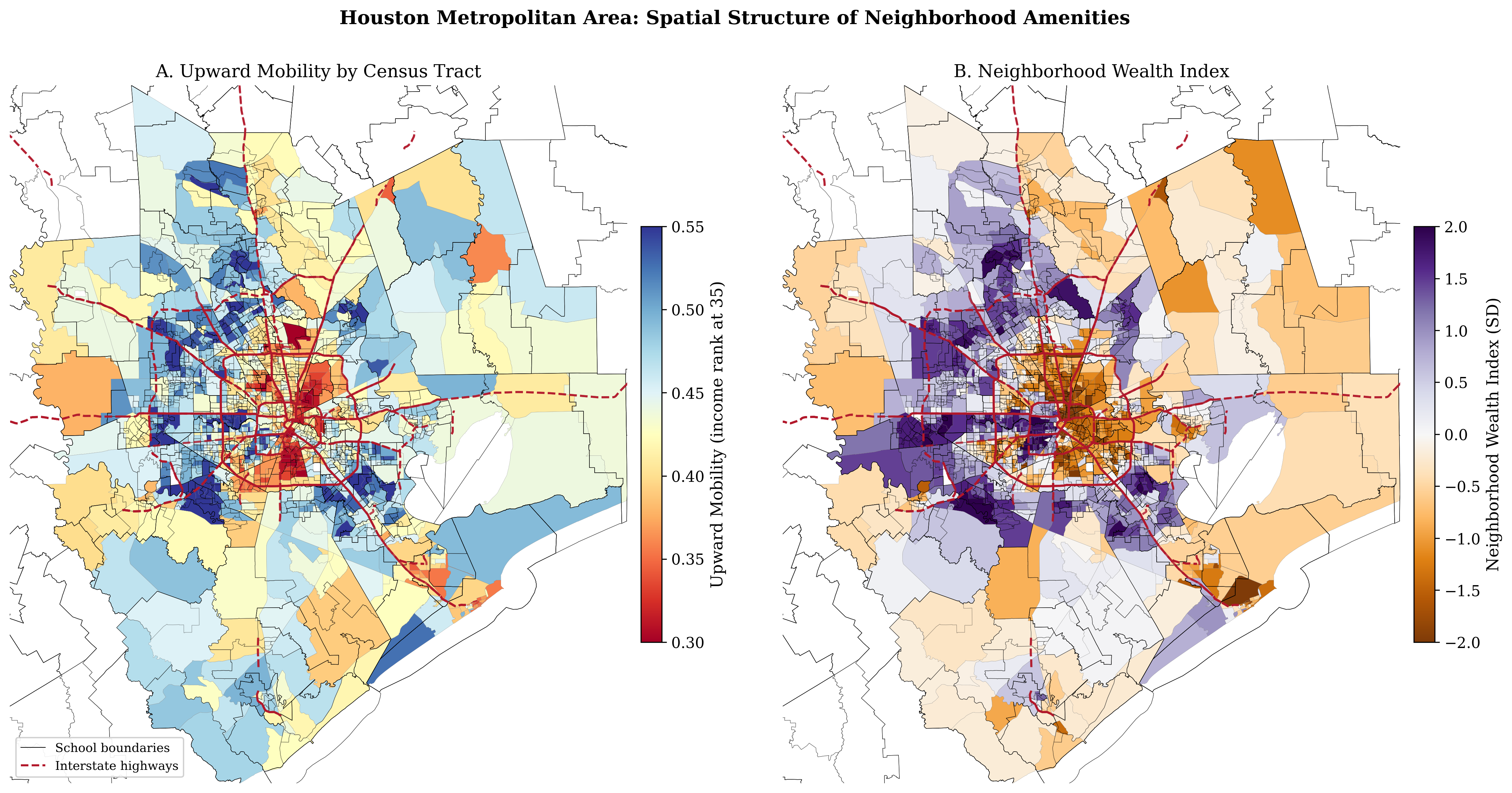
Notes: Panel A: tract-level upward mobility. Panel B: neighborhood wealth index. Thin black lines mark school attendance zone boundaries. Dashed red lines mark Interstate highways.
Outcome Gradients by Amenity Combination
Figure 4 presents upward mobility by school quality and neighborhood wealth quartile, showing near-additivity in raw means that masks genuine complementarity visible in the causal designs.
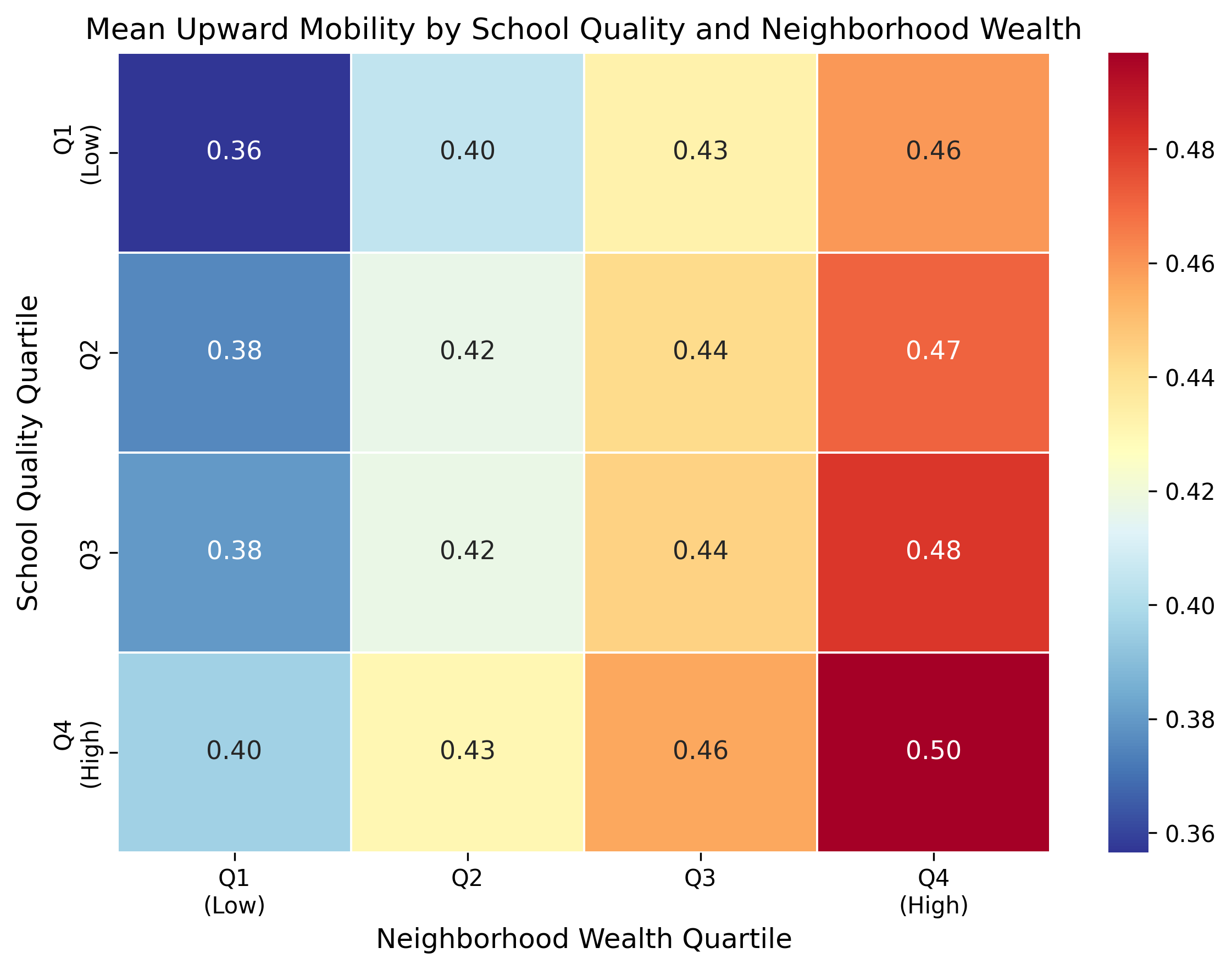
Notes: Each cell shows mean upward mobility for tracts in the corresponding SQ $\times$ W quartile.
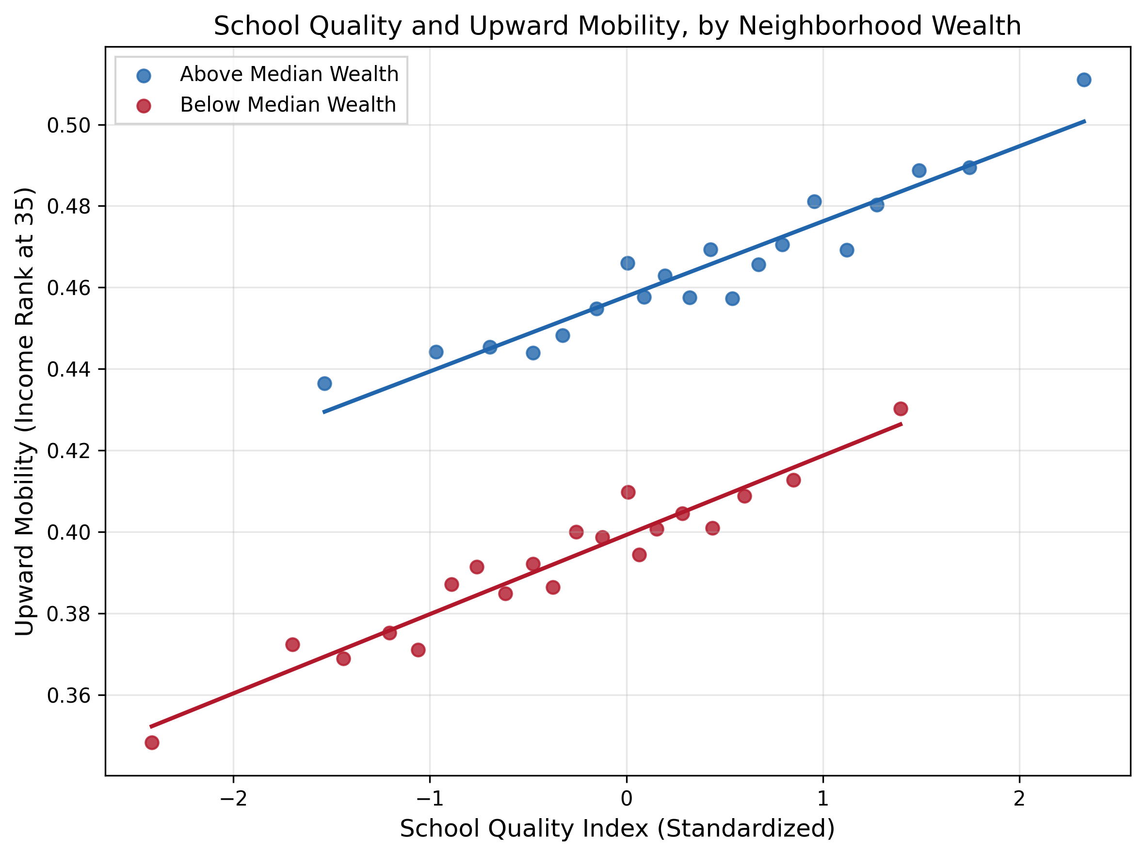
Notes: Each dot is the mean mobility within a ventile of school quality, computed separately for tracts above (blue) and below (red) median wealth.
Spatial Profiles at School Boundaries
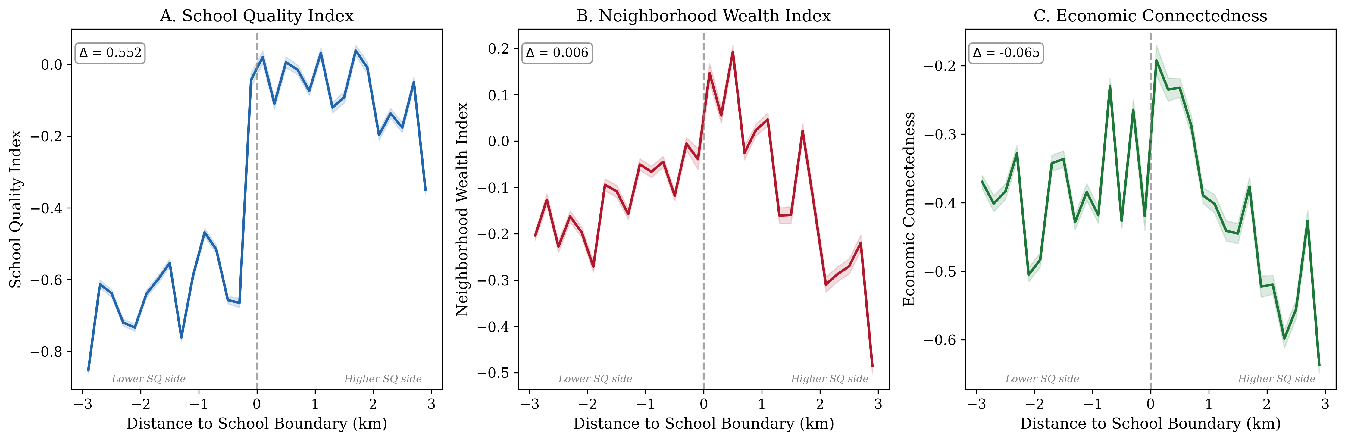
Notes: Average amenity value by signed distance from nearest school boundary, pooled across 86,102 pairs. School quality jumps sharply; wealth and EC vary more smoothly.
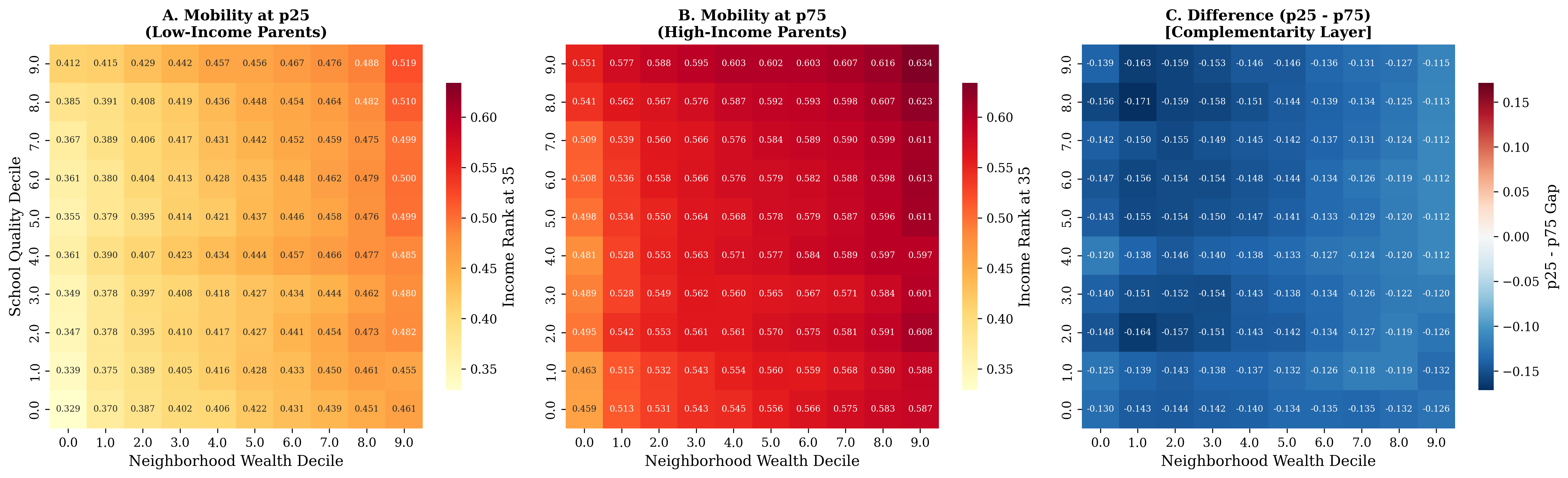
Notes: Each cell shows mean upward mobility in a school quality $\times$ neighborhood wealth decile bin. Panel A: $p25$. Panel B: $p75$. Panel C: difference ($p25 - p75$), showing the complementarity layer.
B. CZ-Level Analysis
The W $\times$ SQ interaction is essentially zero at the CZ level ($-0.001$, $t = -0.21$), but wealth and EC are strong complements ($0.013$, $t = 3.63$).
| (1) No FE | (2) State FE | (3) State FE + Controls | |
|---|---|---|---|
| Wealth ($\beta_W$) | 0.014** (0.007) | 0.009** (0.004) | 0.000 (0.006) |
| School quality ($\beta_S$) | 0.007** (0.003) | 0.012*** (0.004) | 0.010** (0.004) |
| Econ. connectedness ($\beta_C$) | 0.025*** (0.005) | 0.012*** (0.003) | 0.012*** (0.003) |
| W $\times$ SQ ($\gamma_{SW}$) | −0.018** (0.008) | −0.006 (0.005) | −0.001 (0.005) |
| W $\times$ EC ($\gamma_{WC}$) | 0.005 (0.006) | 0.010*** (0.003) | 0.013*** (0.004) |
| SQ $\times$ EC ($\gamma_{SC}$) | 0.010* (0.006) | −0.004 (0.005) | −0.006 (0.005) |
| State FE | No | Yes | Yes |
| Controls | No | No | Yes |
| $N$ (CZs) | 718 | 718 | 718 |
Table 3: CZ-Level Analysis: Amenity Interactions and Upward Mobility
Notes: Dependent variable is mean upward mobility at the CZ level. HC1 standard errors in parentheses.
C. Within-School-Zone Variation
Exploiting variation in wealth and EC within school attendance zones, EC and wealth are substitutes within zones ($\beta_{WC} = -0.005$, $t = -2.40$), while EC complements school quality ($\eta_C = 0.003$).
| (1) Wealth Only | (2) + EC | (3) + Interactions | |
|---|---|---|---|
| Neighborhood wealth ($\beta_W$) | 0.037*** (0.001) | 0.032*** (0.002) | 0.031*** (0.003) |
| Econ. connectedness ($\beta_C$) | 0.017*** (0.004) | 0.018*** (0.004) | |
| Wealth $\times$ EC ($\beta_{WC}$) | −0.005** (0.002) | ||
| Wealth $\times$ School quality ($\eta_W$) | 0.001 (0.001) | ||
| EC $\times$ School quality ($\eta_C$) | 0.003 (0.002) | ||
| School zone FE | Yes | Yes | Yes |
| Controls | Yes | Yes | Yes |
| Observations | 20,501 | 20,501 | 20,501 |
| $R^2$ (within) | 0.262 | 0.280 | 0.284 |
Table 4: Within-School-Zone Variation: Wealth and Social Capital Effects
Notes: School attendance zone fixed effects. Standard errors clustered at zone level.
D. Spatial Decay of Interaction Effects
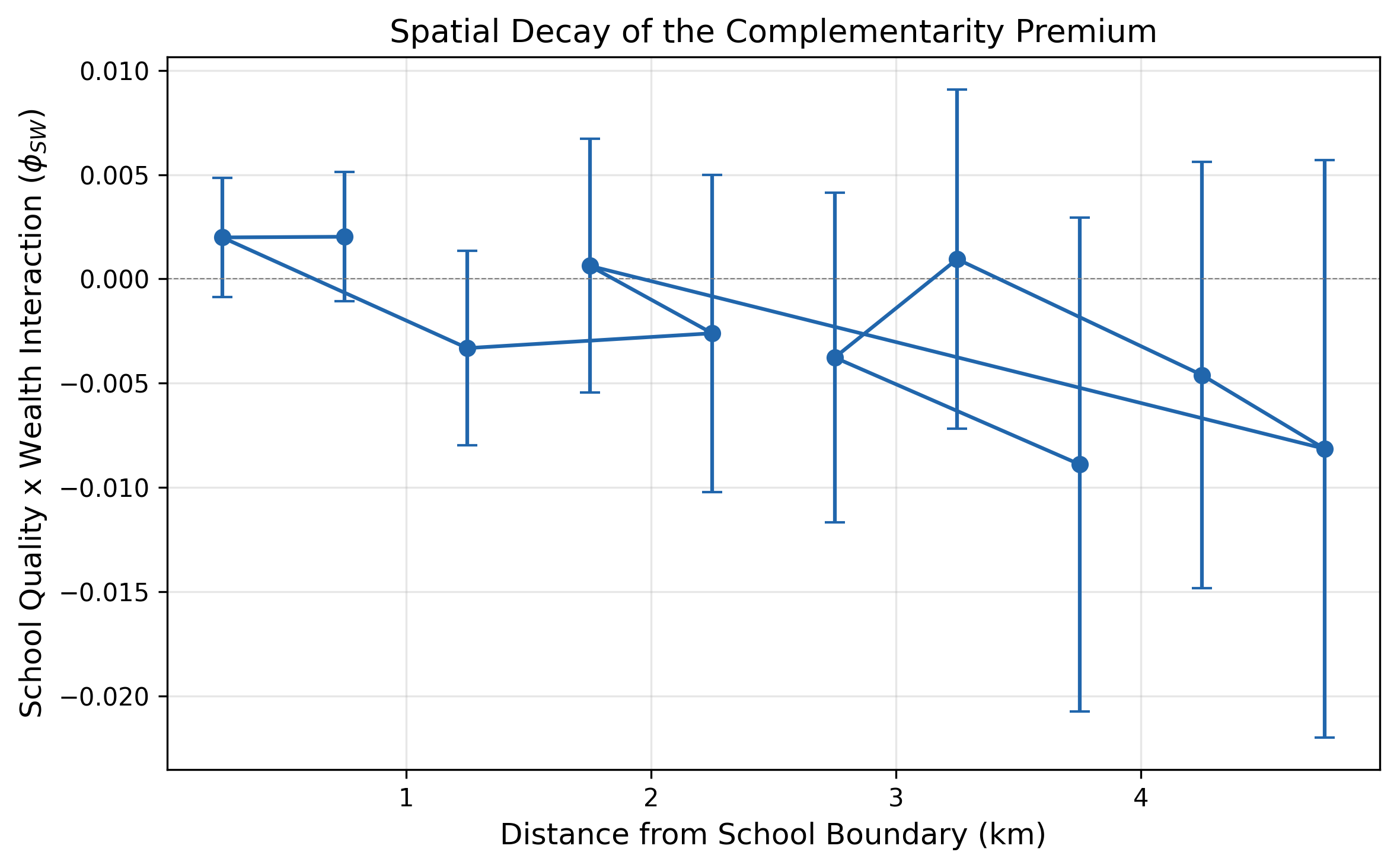
Notes: The interaction coefficient is strongest within 1–2 km and attenuates to zero by approximately 5 km.
E. Variance Decomposition
| Components | $R^2$ | Incremental $R^2$ |
|---|---|---|
| School quality only | 0.401 | 0.401 |
| + Neighborhood wealth | 0.591 | 0.190 |
| + Economic connectedness | 0.601 | 0.011 |
| + All pairwise interactions | 0.602 | 0.001 |
Table 5: Variance Decomposition of Upward Mobility
Notes: Within-CZ $R^2$ with CZ FE and demographic controls. Interaction terms add 0.1 pp of explanatory power beyond main effects.
The interactions add only 0.1 percentage points of explained variance beyond main effects. Their importance lies not in aggregate explanatory power but in the direction and pattern they reveal across the income distribution.
F. Balance Tests
| RD Est. | $t$ | |
|---|---|---|
| Wealth index | 0.226 | (17.74) |
| Median household income ($) | 4,754 | (13.38) |
| Share white | 0.061 | (16.11) |
| Share Black | −0.055 | (−19.61) |
| Poverty rate | −0.027 | (−15.66) |
| Bachelor’s degree+ | 0.041 | (17.63) |
| Economic connectedness | 0.206 | (16.47) |
Table 6: Balance Tests at School Attendance Boundaries
Notes: RD estimates at BW $= 1.0$ km, full sample (86,102 pairs, 691,158 obs). Large imbalances motivate the balanced-pairs restriction ($<0.5$ SD wealth jump).
G. Bandwidth Sensitivity
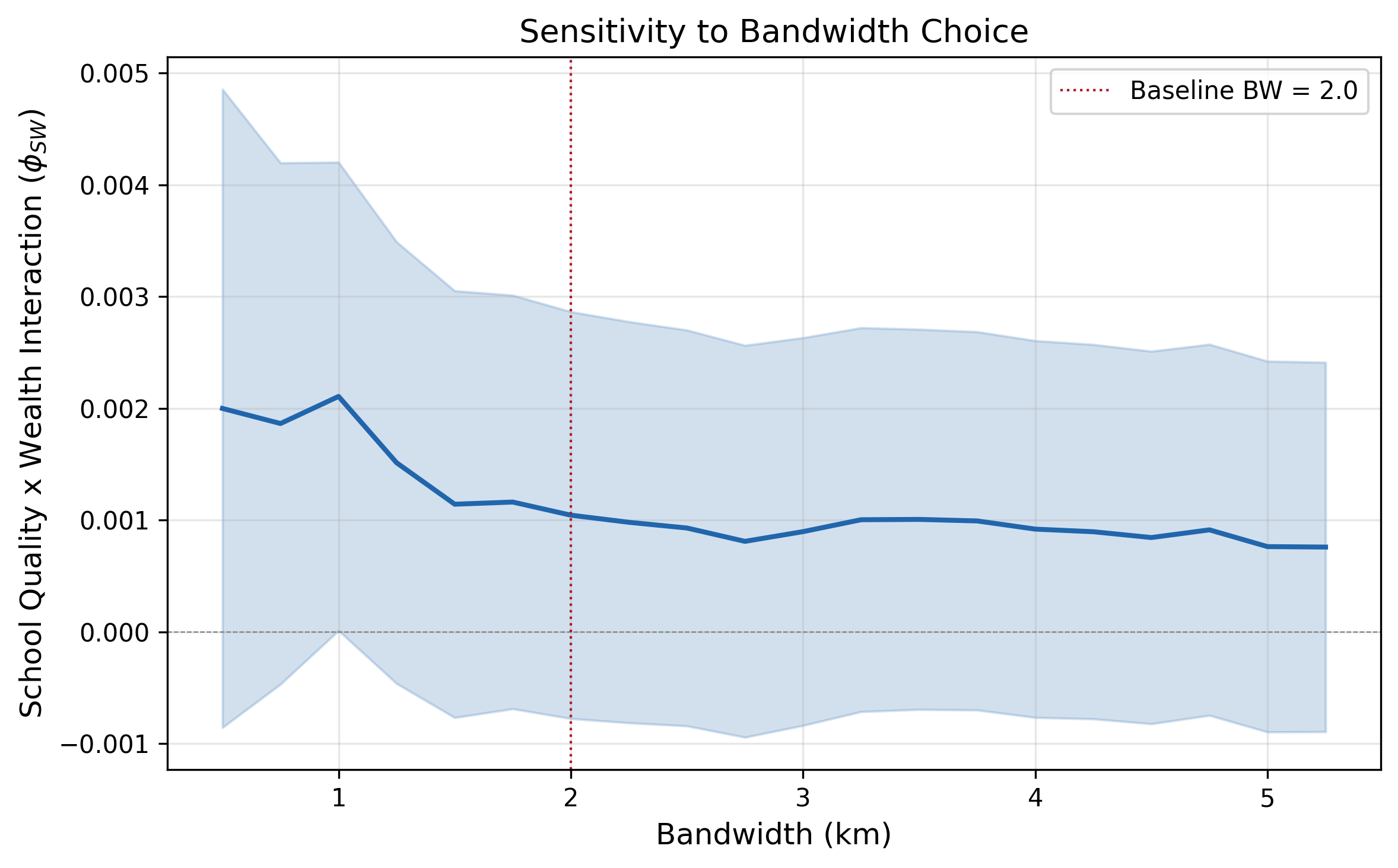
| BW (km) | $\phi_W$ | $t_{\phi_W}$ | $\phi_{EC}$ | $t_{\phi_{EC}}$ | $N$ |
|---|---|---|---|---|---|
| 0.5 | 0.002 | 2.01 | 0.007 | 8.21 | 38,158 |
| 1.0 | 0.006 | 11.08 | 0.006 | 11.87 | 99,578 |
| 1.5 | 0.006 | 14.22 | 0.005 | 12.89 | 152,019 |
| 2.0 | 0.006 | 17.07 | 0.005 | 15.27 | 200,187 |
| 3.0 | 0.006 | 22.81 | 0.006 | 21.20 | 309,520 |
Table 7: School Boundary Pair RD: Bandwidth Sensitivity
Notes: Balanced pairs ($< 0.5$ SD wealth jump). Both interactions positive and significant across all bandwidths $\geq 0.5$ km.
| Estimate | Robust SE | |
|---|---|---|
| Higher-quality school ($\tau$) | 0.025*** | (0.001) |
| MSE-optimal bandwidth (km) | 0.121 | |
| Effective $N$ | 9,915 | |
| Boundary pairs | 86,102 | |
| States | TX, FL, IL, OH, PA |
Table 8: School Attendance Boundary RD (Five States, rdrobust)
Notes: rdrobust with MSE-optimal bandwidth, triangular kernel, bias-corrected robust inference. The basic school quality effect is 2.5 percentile ranks of adult income.
Notes: Panel A: mean upward mobility by distance to school boundary, pooled across five states. Panel B: state-by-state RD estimates with 95% confidence intervals. Sample restricted to balanced boundary pairs.
H. State-by-State School Boundary RD
State-by-state estimates use BW $= 1.0$ km on balanced pairs. SQ $\times$ EC is positive in all five states.
| State | $\tau$ | $t_\tau$ | $\phi_{W}$ | $t_{\phi_W}$ | $\phi_{EC}$ | $t_{\phi_{EC}}$ |
|---|---|---|---|---|---|---|
| Florida | 0.044*** | 5.18 | 0.062*** | 31.15 | 0.033*** | 8.48 |
| Illinois | 0.004* | 1.88 | 0.017*** | 14.10 | 0.015*** | 15.93 |
| Ohio | −0.004* | −1.82 | 0.003*** | 3.35 | 0.002* | 1.85 |
| Pennsylvania | −0.004 | −0.81 | −0.002 | −1.20 | 0.006*** | 3.19 |
| Texas | −0.008*** | −3.20 | −0.000 | −0.41 | 0.003*** | 2.89 |
Table 9: School Boundary Pair RD by State
Notes: BW $= 1.0$ km, balanced pairs. SQ $\times$ EC is positive in all five states.
I. Alternative Outcome Measures
Using a within-zone specification, for incarceration the negative interaction indicates complementarity reduces negative outcomes.
| Outcome | Wealth Effect | Interaction | $t$-stat | $N$ |
|---|---|---|---|---|
| Income rank (pooled, $p25$) | 0.017*** (0.001) | 0.003*** (0.001) | 4.65 | 57,830 |
| Incarceration rate ($p25$) | −0.004*** (0.000) | −0.001*** (0.000) | −2.96 | 57,783 |
| Income rank (male, $p25$) | 0.013*** (0.001) | 0.002*** (0.001) | 3.46 | 57,672 |
| Income rank (female, $p25$) | 0.022*** (0.001) | 0.003*** (0.001) | 4.41 | 57,650 |
Table 10: Alternative Outcomes: W $\times$ SQ Interaction
Notes: Within-zone specification. For incarceration, negative interaction indicates complementarity reduces negative outcomes. HC1 SEs in parentheses.
J. Heterogeneity by Race
Using a within-zone specification with race-specific outcomes at $p25$: stacking white, Black, and Hispanic mobility within each tract, the W $\times$ SQ interaction is positive and significant ($t = 3.24$). The interaction is largest for Black children, consistent with greater amenity-dependence among groups facing larger barriers to private substitution.
| Race | Wealth Effect | Interaction | $t$-stat | $N$ |
|---|---|---|---|---|
| Pooled | 0.017*** | 0.003*** | 4.65 | 57,830 |
| White | 0.018*** | 0.002** | 2.28 | 54,352 |
| Black | 0.010*** | 0.003*** | 2.65 | 27,641 |
| Hispanic | 0.017*** | 0.003** | 2.45 | 28,836 |
Table 11: W $\times$ SQ Interaction by Race
Notes: Within-zone specification, race-specific outcomes at $p25$. HC1 SEs.
| Coefficient | (SE) | |
|---|---|---|
| Black | −0.111*** | (0.003) |
| Hispanic | −0.030*** | (0.004) |
| Wealth | 0.030*** | (0.001) |
| SQ | 0.005*** | (0.000) |
| W $\times$ SQ | 0.002*** | (0.001) |
| W $\times$ SQ $\times$ Black | 0.003*** | (0.001) |
| W $\times$ SQ $\times$ Hispanic | 0.001 | (0.001) |
| CZ FE | Yes | |
| $N$ | 138,271 |
Table 12: Cross-Race Test: W $\times$ SQ Interaction by Race (Stacked Within-Tract)
Notes: Stacking white, Black, and Hispanic mobility at $p25$ within each tract. The W $\times$ SQ interaction is positive and significant ($t = 3.24$). The interaction is largest for Black children, consistent with greater amenity-dependence among groups facing larger barriers to private substitution. CZ-clustered SEs.
K. Grade 3 Math as School Quality
When school quality is measured by grade 3 math scores, results closely replicate the baseline.
| Coefficient | (SE) | |
|---|---|---|
| Black | −0.111*** | (0.003) |
| Hispanic | −0.030*** | (0.004) |
| Wealth | 0.030*** | (0.001) |
| SQ (math) | 0.005*** | (0.000) |
| W $\times$ SQ(math) | 0.002*** | (0.001) |
| W $\times$ SQ(math) $\times$ Black | 0.003*** | (0.001) |
| W $\times$ SQ(math) $\times$ Hispanic | 0.001 | (0.001) |
| CZ FE | Yes | |
| $N$ | 138,271 |
Table 13: Cross-Race Test with Grade 3 Math as School Quality
Notes: School quality measured by grade 3 math scores. Results closely replicate baseline. SEs clustered at CZ level.
L. Placebo and Permutation Tests
We conduct 500 within-CZ permutations, randomly reassigning tract-level amenities within each CZ. The actual W $\times$ SQ coefficient lies 3.0 standard deviations above the null mean, with no permuted coefficient exceeding the actual estimate ($p < 0.002$). See Figure 10. No placebo coefficient exceeds $\mid t \mid = 1.7$ ($N = 71{,}034$ tracts).
| Interaction | $p1$ | $p100$ | Slope | |
|---|---|---|---|---|
| Actual (W $\times$ SQ) | +0.00313*** | −0.00677*** | −0.0000958 | (Real) |
| Placebo: Random $\times$ SQ | −0.00004 | +0.00033 | +0.0000036 | (Flat) |
| Placebo: Random $\times$ W | +0.00026 | −0.00037 | −0.0000061 | (Flat) |
| Placebo: Index $\times$ SQ | +0.00056 | −0.00033 | −0.0000086 | (Flat) |
| EC $\times$ W | +0.00218*** | −0.00830*** | −0.0001013 | (Real) |
Table 14: Placebo Test: Gradient Slope for Real vs. Random Interactions
Notes: Each row reports the interaction coefficient at $p1$ and $p100$, plus the gradient slope. No placebo coefficient exceeds $\mid t \mid = 1.7$. $N = 71{,}034$ tracts.
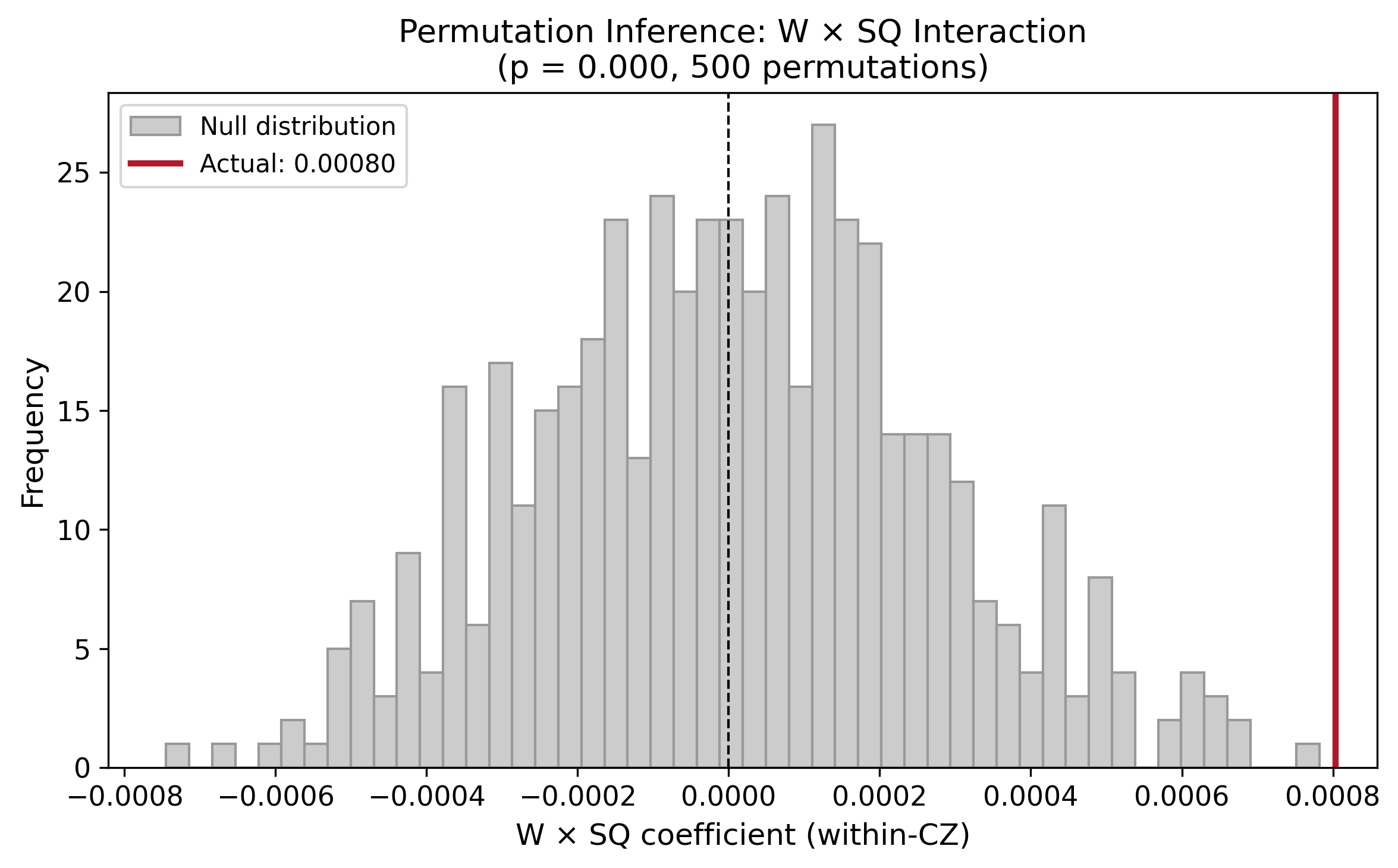
Notes: Histogram shows the distribution of W $\times$ SQ coefficients from 500 within-CZ permutations. Vertical red line marks the actual estimate. $p< 0.002$.
M. Geography of Complementarity
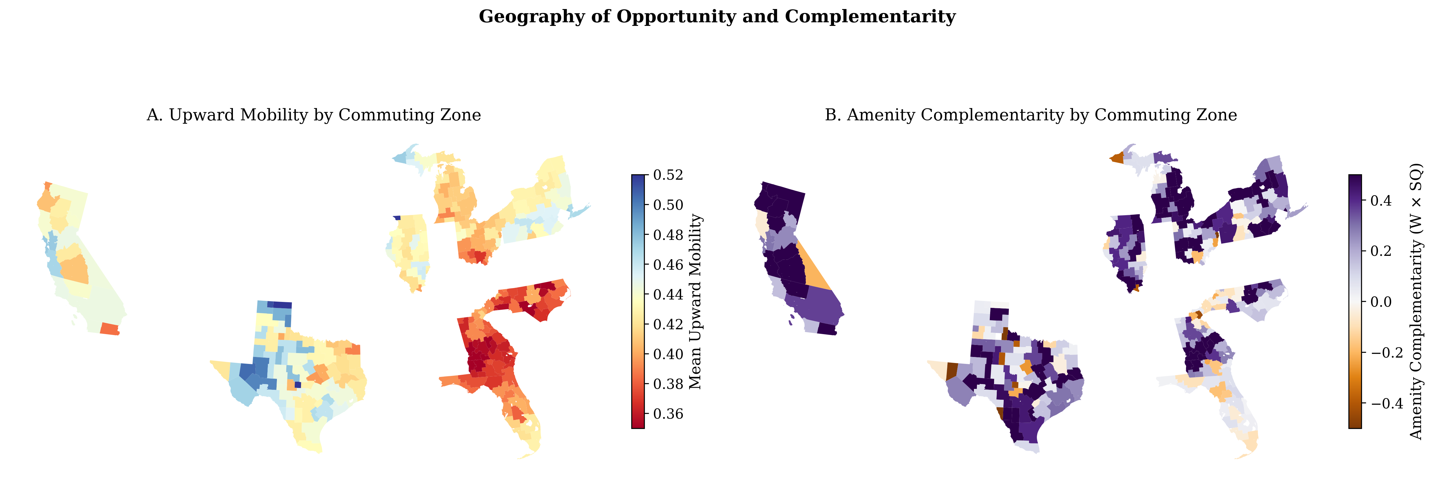
Notes: Panel A: mean upward mobility by CZ. Panel B: CZ-level mean of W $\times$ SQ. Complementary amenity bundles are concentrated in suburban areas of major metropolitan regions.
N. Data Construction Details
School Quality Index
We construct the school quality index from school-level proficiency rates (EDFacts), standardized within state-grade-year cells. For schools with missing data, we impute using student-teacher ratio and per-pupil expenditure via regression imputation.
Spatial Matching
Census tracts are assigned to school attendance zones via spatial join on population-weighted centroids. For tracts straddling boundaries, we assign to the majority-area zone.
Distance Calculations
Distance from tract to boundary is the minimum Euclidean distance from the population-weighted centroid to any boundary polygon point, computed in projected coordinates (UTM).
O. Gender and Incarceration Gradients
Appendix Table 15 reports the cross-percentile gradient separately for male income, female income, and incarceration. The declining gradient replicates for both genders, with the female gradient steeper than the male gradient. The incarceration gradient is positive at every percentile, indicating that complementarity reduces incarceration universally, but is nearly flat across the income distribution.
Panel A: Male Income
| Pctile | W $\times$ SQ | SE | $t$-stat | $N$ | $R^2$ |
|---|---|---|---|---|---|
| $p1$ | +0.00159*** | 0.00031 | 5.19 | 70,817 | 0.243 |
| $p10$ | +0.00070*** | 0.00027 | 2.64 | 70,817 | 0.299 |
| $p25$ | −0.00037 | 0.00023 | −1.62 | 70,817 | 0.370 |
| $p50$ | −0.00216*** | 0.00021 | −10.34 | 70,817 | 0.418 |
| $p75$ | −0.00384*** | 0.00025 | −15.14 | 70,817 | 0.323 |
| $p100$ | −0.00653*** | 0.00039 | −16.70 | 70,817 | 0.152 |
Gradient slope: −0.0000785 ($p < 0.001$). Stacked $p25$ vs $p75$: +0.00386 ($t = 24.3$).
Panel B: Female Income
| Pctile | W $\times$ SQ | SE | $t$-stat | $N$ | $R^2$ |
|---|---|---|---|---|---|
| $p1$ | +0.00484*** | 0.00030 | 15.89 | 70,790 | 0.285 |
| $p10$ | +0.00367*** | 0.00027 | 13.81 | 70,790 | 0.337 |
| $p25$ | +0.00217*** | 0.00023 | 9.57 | 70,790 | 0.409 |
| $p50$ | −0.00037* | 0.00020 | −1.85 | 70,790 | 0.464 |
| $p75$ | −0.00288*** | 0.00024 | −11.81 | 70,790 | 0.363 |
| $p100$ | −0.00688*** | 0.00038 | −17.99 | 70,790 | 0.167 |
Gradient slope: −0.000113 ($p < 0.001$). Stacked $p25$ vs $p75$: +0.00585 ($t = 36.3$).
Panel C: Incarceration Rate
| Pctile | W $\times$ SQ | SE | $t$-stat | $N$ | $R^2$ |
|---|---|---|---|---|---|
| $p1$ | +0.00118*** | 0.00022 | 5.45 | 70,976 | 0.072 |
| $p10$ | +0.00110*** | 0.00014 | 7.75 | 70,976 | 0.094 |
| $p25$ | +0.00104*** | 0.00009 | 11.29 | 70,976 | 0.131 |
| $p50$ | +0.00098*** | 0.00007 | 13.60 | 70,976 | 0.152 |
| $p75$ | +0.00094*** | 0.00008 | 11.49 | 70,976 | 0.078 |
| $p100$ | +0.00092*** | 0.00010 | 9.61 | 70,976 | 0.032 |
Gradient slope: −0.0000024 ($p = 0.006$). Stacked $p25$ vs $p75$: +0.00011 ($t = 1.70$).
Table 15: Cross-Percentile Gradient by Gender and Incarceration
Notes: CZ-FE regressions with HC1 SEs. Gradient slope is OLS of the interaction coefficient on percentile. The female gradient is 45% steeper than the male gradient, and both are monotonically declining. The incarceration interaction is positive at every percentile, indicating complementarity universally reduces incarceration.