Hashing

GRAPHS

A graph is a set of vertices and a set of edges. Here are some examples:

Sometimes you see vertices called nodes and edges called arcs.

A few comments:

In a directed graph (sometimes called a digraph) the direction of the arrow is significant.
For an undirected graph you can go in both directions.
In a directed graph there are sometimes places you can get to but not leave.

Terminology

In the following, there is an edge from vertex 2 to vertex 1:
The two vertices are adjacent
vertex 2 is a predecessor of vertex 1
vertex 1 is a successor of vertex 2

vertices 1 and 3 are adjacent. This is also called being neighbors:

There is a path from vertex 2 to vertex 5: 2, 1, 5. Another path is from vertex 1 to vertex 2: 1, 3, 4, 2 (note you cannot go directly from 1 to 2).

In an acyclic path no vertex is repeated. Above: 1, 3, 4, 2 is an acyclic path. A simple or acyclic graph has only acyclic paths. A directed acyclic graph is often abbreviated as DAG.
A cyclic path has a repeated vertex. Above: 1, 3, 4, 2, 1, 5.

As with circular linked lists, we need to be careful not to keep going around in circles.

A complete graph (undirected) has an edge between every pair of vertices. Thus, every vertex is adjacent to each other:

In some cases a complete graph gives the highest complexity for some algorithms.

a weighted graph has values associated with each edge:

Here, the edge between vertices 2 and 1 has weight 7. The graph can be undirected. Often the weights are restricted to be positive. The weights can represent:

The cost of traversing the edge
The time to traverse the edge
The distance to traverse the edge

An unweighted graph is equivalent to a weighted graph where all edges have a weight of 1.

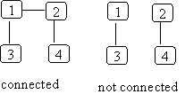
In a connected graph you can get from every vertex to every other vertex (but they don't all have to be adjacent):

A complete graph is always connected (but not visa versa).

Graphs are more general than trees (and therefore linked lists, etc.):

they are nonlinear
you can have as many items connected to as many others as you like
they can have arbitrarily complex connections and cycles

Note: a tree is a restricted kind of DAG.

Uses for Graphs

In general, the vertices represent objects and the edges represent relationships.

airports and flights. The airports (vertices) are objects that are connected by flights (edges):

If vertex j is adjacent to vertex k then there is a flight from j to k

The weight of an edge can be time, distance or cost.

cities and highways

weight is distance or time

tasks to be done

vertices are the tasks and edges represent ordering constraints

Example: CS classes

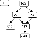
(Note: for illustration only! Don't use to decide what classes to take :-)

statements in a program (flow charts/control-flow graphs)

edges represent flow of control

Representing graphs

Adjacency Matrix

use an V x V array of booleans, where V is the number of vertices in the graph.

array[i][k] == true if there is an edge from vertex i to vertex k

example:

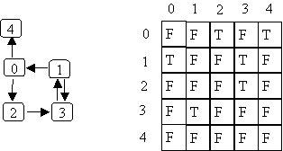
In some situations you can get to yourself (edge from vertex j to vertex j). Here the diagonal can be T.

The matrix is symmetric if undirected graph or always have links in both directions (A[j][k] == A[k][j]).

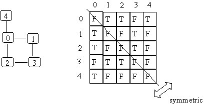
If weighted, the array can hold the weight.

You need a special weight for non-existent edges. If all weights are positive this is easy. If no special value then also need to store boolean to know if edge exists.

2. Adjacency Lists

use a (1 dimensional) array of size V in which each entry is a linked list of adjacent edges.

example:

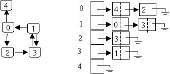
Order in linked list can be arbitrary.

Comparison: Adjacency matrix vs. lists

Operation	Adjacency Matrix	Adjacency List
space	better if dense graph	better if sparse graph
add edge	O(1)	O(1)
remove edge from vertex j to vertex k	O(1)	O(# successors of j) O(V) in worst case
is there an edge from vertex j to vertex k?	O(1)	O(# successors of j) O(V) in worst case
list all successors of a vertex j	O(V)	O(# successors of j) O(V) in worst case
initialize	O(V²)	O(V)

How can you add a vertex?

With an adjacency matrix:

create a new, larger array
copy old values into new array
add values to row & column for new vertex

O(V²)

With an adjacency list

create a new, larger vector (1D array)
copy old value to new vector
add values for new vertex

O(V)

It might seem that making the vector into a linked list would avoid this:

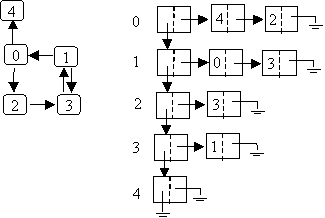
However, you cannot then access a given vertex to look at in O(1) since you have to search down the list.

High-Level Operations on Graphs

As with trees, want to traverse graphs. Two techniques are depth-first and breath-first search. They differ by the order each connected vertex is visited. It is an "orderly" way to traverse (part of) a graph. In each case, the search can differ if begin at a different vertex.

Depth-First Search (DFS)

Variations can be used to answer many questions about a graph:

is it connected?
does it contain a cycle?
is there a path from vertex j to vertex k?
what vertices are reachable from vertex j?
can the vertices be ordered so that for every vertex j, j comes before all of its successors?

You visit one specific successor of a vertex before you visit the other successors. You continue to do this so you go deep, or depth-first, into the graph.

You must keep track of which vertices have been visited to prevent an infinite loop (in a cyclic graph).

Here is the basic algorithm:

start at some vertex v
mark v visited
recursively visit each of v’s successors by repeating steps 2 & 3.

Note: the visited information can be kept in a boolean array of size V where true means visited.

Here is pseudo-code for DFS:

Note: must clear visited at start. You can use a driver method to achieve this.

void dfs (Vertex v) {

visited[v] = true;

for (each successor s of v) {

if (! visited[s]) {

dfs(s);

}

The order in which you visit each successor of a vertex is arbitrary or defined by specific problem.

Since you are using recursion, you are effectively using a stack here.

Here is an example:

The order you visit the vertices is: 0, 2, 3, 1, 4.

If you visited 4 before 2, you would get: 0, 4, 2, 3, 1.

Time for depth-first search:

1 call for each reachable vertex. Each call looks at all successors (even if visited).

time is O(# reachable vertices + # of their outgoing edges)

worst-case = O(all vertices + all edges)

Breadth-First Search (BFS)

Another "orderly" way to visit (part of) a graph.

Some uses:

Can be used to find all vertices reachable from the start vertex (an alternative to depth-first search)
A variant can be used to find the shortest path

Visit all vertices at same distance from start vertex before visiting farther-away vertices. The distance is the number of edges you must traverse.

Uses a queue rather than recursion (which actually uses a stack). The queue holds vertices to be visited. If the graph is a tree, this is like a level-order traversal.

The pseudo-code is:

Note: must clear visited at start. You can use a driver method to achieve this.

void bfs (Vertex v) {

Queue q;

Vertex current;

visited[v] = true;

q.enqueue(v);

while ( !q.empty()) ) {

current = q.dequeue();

for (every successor s of current) {

if ( ! visited[s]) {

visited[s] = true;

q.enqueue(s);

}

Taking the same example as DFS for BFS:

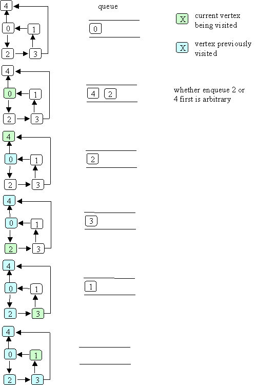
order in which vertices are visited as a result of bfs(0):

The order within a level is arbitrary or problem defined.

As with DFS - all vertices marked visited are reachable from the start vertex but vertices are visited in a different order.

The shortest-path algorithm

Problem: From a starting vertex j find the shortest path (by total weight) to another vertex or all reachable vertices in a graph with positive weights.

This algorithm due to Dijkstra and is sometimes called Dijkstra's shortest-path algorithm.

It finds the absolute shortest path.
There are techniques that are faster to find a path that is close to the shortest path. We won't talk about these.

The method used in this algorithm is how some people do things: lazy but smart:

From the current vertex, go to the next closest one (lazy part).
However, if you were previously at another vertex which has a successor which gives a shorter path then above, use it instead (smart part).

Here is an example:

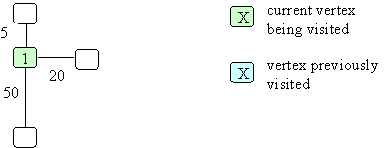
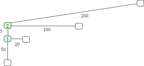
You start a vertex 1. Think of each vertex as being an intersection on a road. At each intersection there is a sign telling you how far it is to the next intersection/location. You don't have a map so you don't know what roads will be at intersections you have not yet visited. As you visit intersections/locations you get more information. From location 1 there are 3 places you can go that are 5, 20 and 50 miles away. Go to the closest location. Why? Without any other information, your best bet is to go to the closest location if you are looking for the shortest path. So being lazy isn't so bad. At this point you have:

From location 2 you realize the closest place is 100 miles away. However, you recall that back at location 1 you could get somewhere in 20 miles. Here is where being smart comes in. You don't just continue down the path you started. You recognize you may have made a mistake and wound up somewhere that isn't likely to lead to a short path. Thus, you decide it would be better to back up to location 1 and continue from there. This gives you:

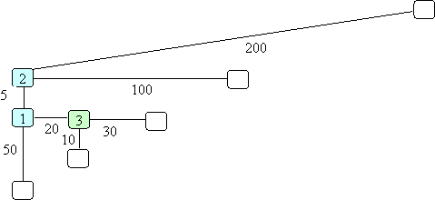
Now you see from location 3 there is a location only 10 miles away so you continue down to there. We could continue with this, but let's first get the details of the algorithm and then do a different example.

The code use 2 arrays of size V (# of vertices)

known boolean array: is shortest path to this vertex known yet?

Once you know the shortest path you don't need to keep trying this vertex.

distance int array: distance to this vertex via known vertices

It is the best path found so far or the best overall if known is true. It has the smallest total weight for all the edges you need to traverse to get here.

Here is pseudo-code for this problem:

// initialize

set all elements of the "known" array to false

set Distance[j] to 0

set all other elements of the Distance array to infinity. Since all distances are positive, you can use -1 to represent infinity.

// main loop

Do {

find the unknown vertex v with the smallest path of all the ones you can consider

set known[v] = true

for (all unknown successors s of v) {

Distance[s] = min (Distance[s], Distance[v] + length of edge between

v and s)

}

The last line is checking if the new path is shorter than the previously shortest path.

To find shortest path from vertex j to vertex k: stop when known[k] == true. You may still determine the shortest path to other vertices (example: Green Bay below).

To find shortest paths from j to all vertices: quit when all vertices are "known", or all unknown vertices have distance == ¥ (they are not reachable from j).

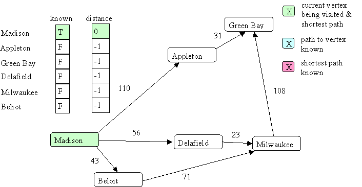
Here is an example where we start at Madison. After initialization:

Now we look at all the successors of Madison:

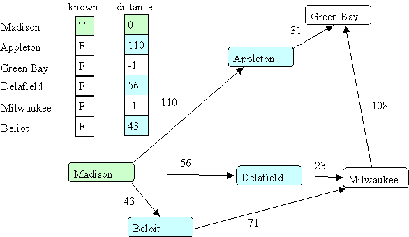
The shortest path that is unknown (excludes Madison) is Beloit, so we go there next and look at its successors:

Next we choose Delafield (Madison & Beloit are now known and excluded):

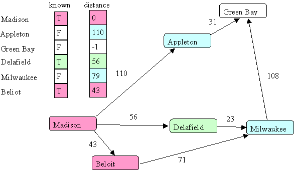
Notice the distance to Milwaukee went down. This is because the initial way through Beloit was farther then the current way through Delafield. This is an example of the fact that following the shortest path doesn't always get you the shortest overall path first. However, you will find it in the end.

Next, we consider Milwaukee:

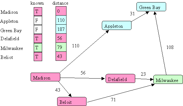
And then Appleton:

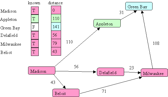
Notice the distance to Green Bay now became 141. Finally, we visit Green Bay:

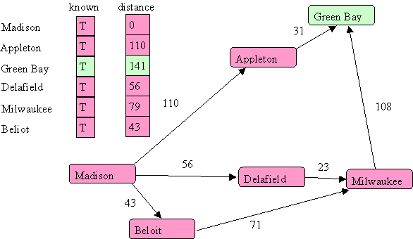
There are no unknown vertices so we are done.

How can you be sure the distance is the shortest one when you mark it known?

You mark the vertex at the end of the shortest path known. Since every other path in the graph is longer and all weights are positive, any new path you determine must be longer. If we allowed negative weights this would not be true. A longer path could get shorter by adding a new edge thereby breaking this algorithm.

How do we know the edges to follow in the shortest path (not just weight)?

Solution: keep track of vertex that lead to each vertex (predecessor).

Replace:

Distance[s] = min (Distance[s], Distance[v] + length of edge between

v and s)

with

if (Distance[s] > Distance[v] + length of edge v and s) {

Distance[s] = Distance[v] + length of edge v and s;

pred[s] = v;

}

The pred array after we visit Madison would be:

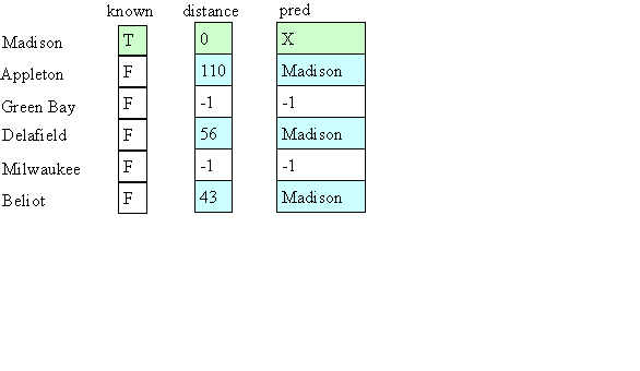
In the end it would look like:

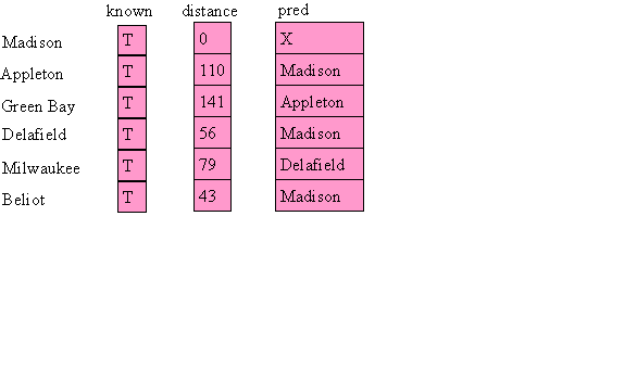
Now you start at your final destination and work backward:

The predecessor of Green Bay is Appleton
The predecessor of Appleton is Madison

This gives:

This is backward to the order we want. You can easily use a stack to reverse the order.

Time for the shortest-path algorithm for a graph with V vertices

The task of finding the shortest path of the available ones is best done with a heap.

In the worst case:

The initialization step takes time O(V)

The main loop

Find unknown vertex v with shortest distance

O(log(E)) if use a heap

Set known[v] = true

O(1)

Set distances of all unknown successors s of v:

O( # edges out of v )

In the worst case, the main loop will execute V times (all vertices’ distances will become known). The complexity depends on whether step 1 or 3 is more expensive. If the graph is dense (complete) then step 3 is O(V) so overall it is O(V²). If the graph is sparse (E < V²) then the complexity is O(Elog(V)). The book has the details.