A binary tree is a BST if for every node in the tree:

• all keys in its left subtree are less than the root (i.e., the key at that node)
• all keys in its right subtree are greater than the root (i.e., the key at that node)

Here are some BSTs:

These are not BSTs:

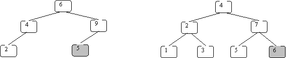
In the left one 5 is not greater than 6. In the right one 6 is not greater than 7.

Note that for a given set of keys, a BST is not unique. It depends on the order in which the items were inserted and deleted:

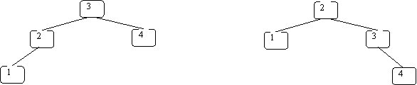
Both of these are valid and have the same keys.

Duplicates add some complications:

• can store as separate nodes and make less than into less than or equal or greater than into greater than or equal

• can store all the same keys within one node

We won’t deal with duplicates.

As with most ADTs we want to add, remove and find.

A BST is related to a binary search on a sorted array. Recall you keep looking at the middle item of the part of the array remaining to consider and then go left or right depending on whether the item being searched is smaller or larger. This was worst case O(log(n)). The problem was that adding and removing was O(n) due to the shifts. A BST will get us O(log(n)) for the search (in most cases) as well as O(log(n)) for add/remove (in most cases). However, in the worst case it is O(n) for these.

Searching

The find operation is called searching. Because of the structure of the binary tree, you have useful information. At each node, you can compare the key you are looking for with key at the node. Here are the possibilities:

• The keys are equal: You have found the desired item.
• The search key is less than the key at this node. The item (if it is in the tree) is to the left. Recursively search the left subtree.
• The search key is greater than the key at this node. The item (if it is in the tree) is to the right. Recursively search the right subtree.

Before you do the last two items you need to make sure the left or right subtree is not empty. If it is then the search fails.

Let’s use the following BST:

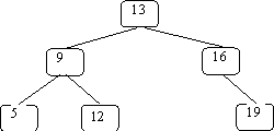
and search for 12:

What if we search for 15:

How much work does it take to search for an item?

To find an item at depth d means looking at d + 1 nodes (recall depth is the number of edges traversed).

In the worst case you have to go all the way to a leaf to realize the item is not there. The height of the tree would be the longest path. You visit one more node than the height (which is the number of edges) assuming you don’t count recognizing the child is null.

As is typical with a binary tree, the worst case complexity is the height of the tree (dropping the +1).

What is the height? We will discuss this in more detail later but for now let’s take a good case: suppose the tree is full. This is good because you have the smallest height of the tree for the number of nodes. Recall it looks like:

This looks just like the divide stages picture from the merge sort discussion.

Using similar logic you can show that the height of the tree is é log₂(n)ù where é xù is the smallest integer greater than or equal to x.

Thus, the worst case complexity for a BST that is a full binary tree is O(log(n)). We will see later that the worst case for any BST is O(n).

Add/Insert

Where should a new item go in a BST?

The answer is easy: it needs to go where you would have found it!

If you don’t put it there then you cannot find it later.

This turns out to be very easy since all unsuccessful searches end by seeing a null child of node. Adding something here is very easy – just change the null reference to the new node in the tree.

Here are the steps:

• search for the key of the item:
• if you find it, deal with the duplicate. For now just assume you replace the old item with the new one (you don’t allow duplicate keys in this BST).
• If you don’t, you are sitting at the null reference to a child of a node. Replace it with a reference to the node to insert.

Let’s insert 15 into the BST from before. The search steps are the same:

It is easy to see that the complexity is the same as with search.

Delete

As you would expect, deleting an item involves a search to locate the item. If the search fails then so does the delete.

If you find the item, there are several cases to deal with:

1. It is a leaf so it has no children
2. It has one child
3. It has two children

The reason we have to be careful is just like linked lists we do not want to orphan any nodes when we remove one.

1. Node to delete is a leaf without children

This case is easy. Since it has no children you can simply remove it from the BST. As an example, suppose we remove item with key 15 that we added before (the search is not shown):

 



Keep in mind you need a reference to the parent of the node to delete (16 in the example) to remove the child. This is because you must remove this child from the parent. This isn’t hard: just stop the one level sooner or keep a reference to the previously considered node. All the delete cases need this.

2. Node to delete has one child

This isn’t much harder. Because of the recursive nature of BSTs, you can simply replace the parent with the child.

As an example, let’s delete 16 from the BST just formed:

 



 

3. Node to delete has two children

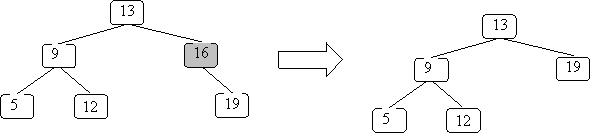
This case is a little harder. You cannot simply pick one of the children to replace the parent. It might already have two children so it cannot add the other child on. For example, if you want to remove 13 above and replace it with 9, then 9 would need to have 3 children: 5, 12, and 19. This is not allowed.

The trick is to change the problem into an easy one. In this case we replace the node we want to delete with a node with 0 or 1 child. Then we can easily delete the original copy that is now a duplicate.

The question is what node can we use to replace the one to delete?

As mentioned before, a BST has some structure but that does not uniquely define the exact representation of the ADT. This gives us a chance to find a replacement as long as we follow the BST structure.

The rule is that every node in the left subtree is smaller and every node in the right subtree is larger. This gives us two possibilities to replace the node:

• The largest node in the left subtree of the node to delete. This is also smaller than any node in the right subtree because it came from the left subtree.
• The smallest node in the right subtree of the node to delete. This is also larger than any node in the left subtree because it came from the right subtree.

Either one is fine. The book uses the second one (smallest node in the right subtree) so I’ll use that.

Now that we know what node to use, how can we find it?

The structure of a BST tells us that the smaller value is to the left. Thus, you follow left children as far as you can in the right subtree to find the smallest value.

Hopefully you can convince yourself that you only need to go down the tree at most once. In the first two cases you do a find and a couple of operations to remove the node. In the third case you do a find and then step down the right subtree. This isn’t farther than the height of the tree. Then you do a few steps to replace and delete. Thus, the overall complexity is the height of the tree in the worst case.

General discussion of complexity

If the tree is full, then the height is log(n) so the complexity of these operations is O(log(n)). However, you can get much worse.

Previously with sorting, we often checked what happens if you tried to sort sorted data. Let’s insert sorted data into a BST. You get:

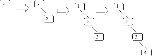
It is pretty easy to see you get all right children. If you use reverse sorted data you get all left children. The height of the tree is n so all the operations become O(n) in the worst case. This is expected since this is basically a linked list.

The book shows that for randomly assembled BSTs the average height of the tree is 1.38* log(n). Thus, you expect the average complexity for these operations to be O(log(n)). This seems to be the case in practice but has not been shown analytically since the remove operation can change the height from the random assembly case.

This discussion shows that if the BST becomes unbalanced (large height) then the complexity is much worse than the good case of log(n). The next topic we will discuss is balanced binary search trees, which avoid this problem.

Before we do that, a few points:

• With binary search of an array, the search was always O(log(n)). However, the insert and delete required a shift of the array and is O(n) on average. In a BST you can do insert, delete and search in the best case (and can also expect the average case) in O(log(n)). This gives us the change operations (add and delete) with a low complexity. However, the worst case is O(n) for all of these. This makes the search worse than a sorted array in the worst case. Notice a BST has less structure than a sorted array.
• If you do an inorder traversal of a BST the data comes out in sorted order. Assuming you don’t get a bad case, the complexity for inserting n items into a BST is O(nlog(n)). The traversal is O(n). The overall complexity is O(nlog(n)) which is the same as our other good sorting algorithms. However, the worst case is not as good (O(n²)) and it is usually slower even in the good cases. Trying this makes a good exercise.
• To copy a BST you can do a preorder traversal and insert the items in this order into a new BST. Again, this makes a good exercise. However, the complexity is now O(nlog(n)) in the good cases because you do n inserts in the new BST.