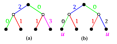
If a tree vertex x which has been a tree leaf embedded into hypercube node \varphi(x), becomes a parent of one or two children, it generates its flip bit and performs the following steps:
if \fb(x)=0 then
|
embed left son (if it exists) back into \varphi(x);
|
embed right son (if it exists) into \varphi(x)\XOR t(x);
|
else
|
embed left son (if it exists) into \varphi(x)\XOR t(x);
|
embed right son (if it exists) back into \varphi(x).
This simple approach gives surprisingly good results. For an M-vertex binary tree and an N-node hypercube, it achieves \dil=1 and \load=O(M/N+log N) with high probability.
Simulation of binary Divide&Conquer computation on a hypercube
Many problems lead to the following binary parallel n-level Divide&Conquer (D&C) computation:
- the root process splits the problem (input data) into two halves and passes them to its two children,
- the children do recursively the same,
- at level n, the granularity of subproblems is small enough to be solved be leaf processes,
- results are recursively moved back to the root which combines them into the final result.
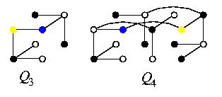
We may use a standard embedding of CBTn in Qn+1 with \load=1 (see Subsection \ref{StaticTreestoQ}) to simulate such a computation on Qn+1, but it would be inefficient, since one half of hypercube nodes, simulating the internal vertices of CBTn, would idle most of the time. However, there is a trivial method how to simulate such a computation optimally on Qn.

CAPTION: Simulation of 3-level D&C computation on Q3.
- the root node splits the problem (input data) into two halves,
- it hands over one half to its neighbor in dimension 0 and retains the other half,
- both these two nodes are active and do the same with their halves using dimension 1,
- this is repeated for dimensions i=2,...,n,
- all the nodes of Qn become leaves of CBTn and compute the leaf subproblems,
- results are folded back in the reverse order.
This corresponds to an embedding of CBTn into Qn as shown on Figure(a). Left children are mapped onto the same hypercube node as their parents. The embedded tree forms so called binomial spanning tree of the hypercube (see Figure(b)), which we will see again in Section 10 of this course.
Embeddings of meshes-of-trees
Even though it is known that MTn is even a subgraph of Q2n+2 (which is the optimal hypercube), we will only explain here an easy way how to embed MTn into Q2n+2 using the results above. We just use these three facts:
- Q2n+2=Qn+1 × Qn+1,
- MTn\subsetCBTn× CBTn,
- CBTn can be embedded into Qn+1 with \dil=2 and \load=\ecng=1 (see Subsection \ref{StaticTreestoQ})).
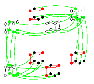
This gives immediately an embedding of MTn into Q2n+2 with \dil=2 and \load=\ecng=1:
- embed CBTn into Qn+1 with \dil=2 and \load=\ecng=1,
- apply cartesian product to get an embedding of CBTn× CBTn into Q2n+2
with \dil=2 and \load=\ecng=1,
- convert CBTn× CBTn into MTn by removing superfluous edges.

CAPTION: MT2 embedded in Q6 with \load=\ecng=1 and \dil=2.
Embeddings of meshes
Again, the basic approach takes advantage of the fact that the hypercube and the meshes are defined recursively as cartesian products of lower-dimensional hypercubes and meshes, respectively.
- Linear array M(z) is a subgraph of its optimal hypercube Qn using any Gray code, where n=[log z].
- M(2n1, 2n2,..,2nk), ni>=1, is a spanning subgraph of Qn, n=n1+...+nk. The construction is trivial just by embedding each M(zi) into corresponding Qni, where ni=[log zi], and by applying cartesian product to the results. This can be generalized:
- If [log z1]+...+[log zk]=[log(z1... zk)], then M(z1,.., zk) is a subgraph of its optimal hypercube Qn, where n=[log(z1... zk)]. Algebraically, this mapping is computed as follows:
|
A vertex (x1,...,xk) of M(z1,...,zk), 0<= xi<= zi-1, is mapped into Qn to node
Gl1(\binl1(x1))\circ Gl2(\binl2(x2))\circ... \circ Glk(\binlk(xk)),
where
- \binm(x) denotes m-bit binary representation of integer x < 2m,
- li=[log zi],
- Gl is BRGC encoding on l bits, defined on Page,
- \circ is string concatenation.
If [log z1]+...+[log zk] > [log(z1... zk)], this ``cartesian decomposition'' method gives embeddings with \vexp > 2, thus not optimal. To achieve optimality, more sophisticated methods must be used. We state just some results here.
Any 2-D mesh M(a,b) such that [log a]+[log b]=[log(ab)]+1 can be embedded into its optimal hypercube Q[log(ab)] with \load=1 and \dil=\ecng=\vcng=2.
A similar best known algorithm for 3-D meshes gives embedding with dilation 5.
Embeddings of higher-dimensional meshes into optimal hypercubes with load one and minimal dilation are still an open problem. The best known result is that n-dimensional mesh can be embedded with \dil=4n+1.
Embeddings of hypercubic networks
Embeddings of other graphs
- Given graph G and integers k and n, the problem of embedding G into Qn with dilation k is known to be NP-complete.
- Embeddings of de Bruijn graphs with constant dilation and expansion into the hypercube are not known.
Embeddings into meshes and tori
2-D or 3-D meshes/tori are currently the most commonly used IN topologies, therefore methods how to embed other networks into them or how to simulate them on them are of high practical interest.
Lemma
Given a graph G, integers k and n, the problem to embed G into an n-dimensional mesh with \dil<= k is NP-complete\comment{\cite{bhattcosmakis}}. This holds even for k=1, n=2, and G = binary tree.
On the other hand, problems of embeddings into 2-D meshes are very close to problems of designing VLSI layouts and many solutions/approaches are known\comment{\cite{ullman}}.
Embeddings among meshes and tori
Lemma
Meshes and tori are computationally equivalent, since they are quasiisometric.
Proof
Given integers z1,...,zn, let M=M(z1,...,zn) and T=T(z1,...,zn).
- M is a subgraph of T so that T can simulate M with no slowdown.
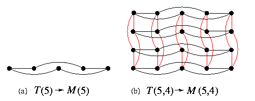
- On the other hand, T can be embedded into M with \load=1 and \dil=\ecng=2.
- Decompose M into cartesian product M(z1)× ...× M(zn) and T into T(z1)× ...× T(zn).
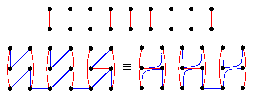
- Embed each cycle T(zi) into M(zi) with \load=1 and \dil=\ecng=2 as shown on Figure(a) for z1=5.
- The embedding of T into M is composed by using the cartesian product. Figure(b) shows 2-dimensional case.

CAPTION: Optimal embedding of tori into meshes with \load=1 and \dil=\ecng=2.
If the mesh and torus do not have the same dimensionality or side lengths, we first embed tori into tori or meshes into meshes and then apply this solution.
Embeddings of tori into tori
In case of general higher-dimensional rectangular and cube tori, the problem of optimal embeddings is hard and open. Optimal solutions are known only for special low-dimensional cases. We will mention one such result.
Lemma
Let z1\not=z2. Then 2-D torus T(z1,z2) can be embedded into cycle T(z1z2) with \load=1 and with optimal \dil=\ecng=min(z1,z2).
Proof
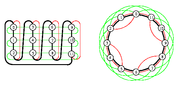
The embedding is simple and straightforward: it is based on one-to-one vertex mapping of T(z1,z2) which is either row-major if z1>= z2 or column-major otherwise. See Figure for an example.

CAPTION: Optimal embedding of 2-D torus T(3,4) into cycle T(12) with \dil=3=min(3,4) based on column-major vertex mapping. Horizontal edges of T(3,4) have \dil=3 and vertical wrap-around edges have \dil=2.
Embeddings of meshes into meshes
Here we will explain some methods how meshes can simulate each other if they are of the same size but differ in the number of dimensions and/or the lengths of sides. It is again a difficult problem in general, we will discuss only several special cases for which solutions are known. A mesh with nonequal side lengths is called rectangular here. The notation for cube meshes will indicate the dimensionality with a subscript at M. For example, Md(w,...,w) denotes a d-dimensional cube mesh.
Embeddings of cube meshes into rectangular meshes
Theorem
Let n>= 2 and let z1>= ...>= zn>= 2 be different integers. Let N=\Pii=1n zi, w=N1/ n, R=M(z1,...,zn), and S=Mn(w,...,w). Without loss of generality, assume that w is integer. Then
R can simulate S with slowdown {maxi zi/ w}.
Proof
Inductive by showing that there exists an embedding of S into R with \dil=\ecng=O((maxi zi)/w) and constant load.
- (i) Induction basis:
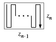
- Let n=2 and z1 > z2. Then S=M(w,w) can be embedded into R=M(z1,z2) with \dil=[ z1/w], \load=2, and \ecng=O([ z1/w]). We show here one possible solution, but there are other ones with similar properties. Columns of S are placed successively into R left-to-right along the first dimension besides each other without overlapping. Each of them starts in the first row of R and snakes vertically through R rightward. See Figure. Since some nodes of R are wasted, the last column of R is reached before all columns of S are embedded, but in that case the snaking simply bounces mirror-like back. Some nodes of R will have \load=2 and some \load=0. The width of one snake in R is [ w/z2]=[ z1/w]=[max(z1,z2)/w] and this is the dilation of horizontal edges of S and link congestion of horizontal links in R is 1+z1/w.

CAPTION: Embedding of a 2-D square mesh into a 2-D rectangular mesh.
- (ii) Auxiliary lemma:
- \
Lemma
M(z1,...,zn-2,zn-1zn) is a subgraph of M(z1,...,zn-1,zn).
Proof
We use again a simple snake-like embedding. M(zn-1zn) can be snaked through M(zn-1, zn) with unit measures as shown on Figure and the general case follows from the cartesian-product property.

CAPTION: Snaking M(zn-1zn) through 2-dimensional M(zn-1,zn).
- (iii) Induction step:
- Decompose R into w submeshes Ri=M([ z1/w],z2,...,zn), i=1,...,w, and S into w submeshes Si=Mn(1,w,...,w). The embedding of S into R is composed of one-to-one embeddings of Si into Ri along the direction of z1 in R (see Figure). Since the width of Ri along the first dimension is [ z1/w], the edges in the first dimension of S have dilation [ z1/w]. Individual embeddings of Si into Ri for i=1,...,w are by induction. Since each Si is isomorphic to an (n-1)-dimensional cube mesh Mn-1(w,...,w), we can embed it by induction into (n-1)-dimensional mesh M([ z1zn/w],z2,...,zn-1) with dilation
[{max([ z1zn/w],z2)/ w}]<=[ z1/w],
\ecng=O(z1/w), and \load=2. By Lemma, (n-1)-dimensional mesh M([ z1 zn/w], z2, ...,zn-1) is a subgraph of n-dimensional mesh Ri=M([ z1/w],z2,...,zn). It follows that each Si can be embedded into Ri with \dil=[ z1/w], \ecng=O(z1/w), and \load=2.

CAPTION: Recursive embedding of n-dimensional S into R.
Corollary
S can be simulated by (n-k)-dimensional mesh Mn-k(N1 / n-k,...,N1 / n-k) with slowdown Nk / n(n-k).
Proof
By Theorem, S can be embedded into R=Mn(N1 / n-k,...,N1 / n-k,1,...,1) with dilation
{N1 / n-k/ N1 / n}=Nk / n(n-k)
and R is isomorphic to (n-k)-dimensional Mn-k(N1 / n-k,...,N1 / n-k).
Embeddings of rectangular meshes into cube meshes
Theorem
Let R and S be meshes defined as in Theorem. Then
R can be embedded into S with constant dilation.
Proof
|
- (i) Induction basis:
- Let n=2. Then R=M(z1,z2) can be embedded into S=M(w,w) with \dil=1 and \load=\ecng=2 by a trivial snaking combined with perpendicular overlap bending at vertical boundaries of S as shown on Figure. Note that the nodes of S close to its vertical boundaries have \load=0 or \load=2.

CAPTION: Embedding of M(z1,z2) into M(w,w) with \dil=1.
- (ii) Induction step:
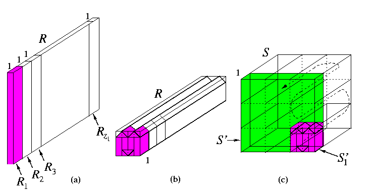
- Let R'=M(z2,...,zn), S'=Mn-1(w,...,w), r=|V(R')|, and s=|V(S')|. Since z1 > w, it follows that r={N / z1} < s={N / w}. Thus {s / r}=z1/w > 1. By definition, R=M(z1)× R' and S=M(w)× S'. We split (n-1)-dimensional mesh S' into [{s / r}] cube submeshes Si'=Mn-1(r1 / n-1,...,r1 / n-1) (Figure(c)). R can be split along the first dimension into z1 (n-1)-dimensional submeshes Ri, isomorphic with R', i.e., of size r each (Figure(a)).

CAPTION: Embedding of n-dimensional rectangular mesh into d-dimensional cube mesh with \dil=1.
By induction, R1 can be embedded into S1' with unit dilation. The rest of mesh R is reshaped in the same way so that R can be viewed as a mesh Mn(z1,r1 / n-1,...,r1 / n-1) (Figure(b)). This folded mesh is then snaked through S in the way depicted in Figure(c).
Embeddings among 2-D rectangular meshes
A practically important problem is embedding of one 2-D mesh into another one of approximately the same size with \load=1. There exist some partial solutions\comment{\cite{ellis}}. We will not describe the methods here due to the lack of space. They are usually based on small primitive tiles from which embeddings of larger meshes are constructed by composing, squeezing, and folding.
Lemma
Consider M(a,b) and M(a',b') such that a' < a<= b and b' is the minimum integer satisfying a'b'>= ab.
- This result is optimal, since the lower bounds on dilation and congestion are 2.
- If a/a'<= 2, then M(a,b) can be embedded into M(a',b') with \dil<=2.
- If a/a'<= 3, then M(a,b) can be embedded into M(a',b') with \dil<=3.

CAPTION: Embedding of M(2,9) into M(3,6) with \dil=2 and \ecng=3.
Simulation of parallel binary D&C computation on 2-D meshes
Lemma
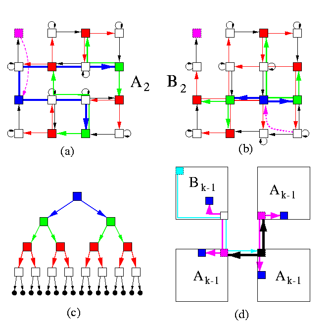
CBT2m can be embedded into M(2m,2m) with bidirectional links so that
- \load=2: Each mesh node is loaded with exactly one leaf vertex and (except one) exactly one internal vertex
- distinct tree edges are mapped on arc-disjoint links in the mesh
- \dil=2m+O(m)
Proof
The embedding is again nicely recursive. The basic idea follows from Figure. The induction base is in parts (a)-(c). Part (c) shows CBT4, which is embedded in M(22,22) using either pattern A or B. Note than in each pattern, one node is loaded with only one leaf and can therefore become a new root when building larger trees from these building blocks. Also there are some free arcs which can be used for joining subtrees to new roots. Part (d) illustrates the induction step.

CAPTION: Simulation of D&C computation on a square mesh.
Embeddings of linear arrays and cycles into high-dimensional meshes and tori
- Hamiltonian paths/cycles:
- We have seen in Section 5 that
- any T(z1,...,zn) has a hamiltonian cycle,
- any M(z1,...,zn) has a hamiltonian path,
- M(z1,...,zn) has a hamiltonian cycle iff at least one zi is even.
- Recursive patterns:
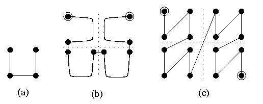
- Cube meshes Mn(k,...,k), where k=2i for some integer i have hamiltonian paths/cycles with a nicely recursive structure. Let us demonstrate for 2-D mesh Mi=M(2i,2i) one solution which is suitable for example for mesh-of-trees or pyramidal meshes.
- Induction base:
- M1 is trivial (see Figure(a)).
- Induction step:
-
- split Mi into four quarters Mi-1,
- construct hamiltonian path recursively in each of them, so that the upper two patterns are rotated by 90 degrees as shown in Figure(b),
- join the terminal vertices of these paths as shown in the same figure.
- Peano curves:
- If large dilation is not an issue (for example in case of distance insensitive routing), meshes can be traversed in a fractal-like way. Very useful are so called Peano curves (see Figure(c)). They have dilation \dil=\Theta(\sqrt{N}), but their fractal structure does not require rotation, it needs just a translation.

CAPTION: Recursive numbering schemes for square 2-D meshes.
Embedding linear arrays/cycles into any network
Linear arrays and cycles as the most trivial topologies can be embedded with constant measures into any network, this is a classical result by Sekanina\comment{\cite{sekanina}}.
\begin{lemma}
An N-vertex cycle C can be embedded into any N-node network G with \load=1, \dil<= 3, and \ecng=2.
\end{lemma}
Proof
Constructive
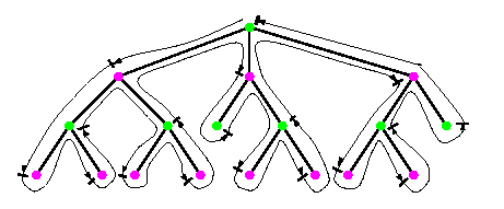
- construct a spanning tree TG of G,
- partition its nodes into two classes V0 = nodes at even-numbered levels of TG and V1 = nodes at odd-numbered levels of TG,
- embed C in G by traversing TG in the depth-first order and by placing vertices of C into nodes of TG using the following rule:
- the currently visited node x of TG is in V1 and it is our first visit of x,
- the currently visited node x of TG is in V0 and it is our last visit of x.
Each node of TG will be loaded exactly once. The proof that \dil=3 follows from the recursive structure of any spanning tree.

CAPTION: Embedding an N-vertex cycle into N-node network G with \dil=3 and \load=1.
Embeddings into hypercubic topologies
Lemma
Both types of butterflies and CCC are computationally equivalent.
Proof
- CCCn is a spanning subgraph of wBFn.
-
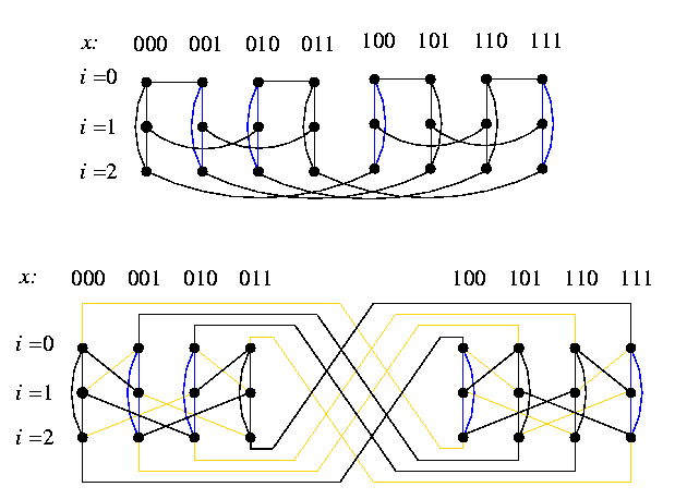
The embedding is based on a one-to-one vertex mapping \varphi:V(CCCn)-> V(wBFn) defined as \varphi((i,x))=(i+n \parity(x),x), where \parity(x) returns 1 if x has odd parity, and 0 otherwise. Rotation of all odd-numbered cycles of CCCn by one position forward gets them into the same position as in wBFn.

CAPTION: CCC3 (thick lines) spans wBF3.
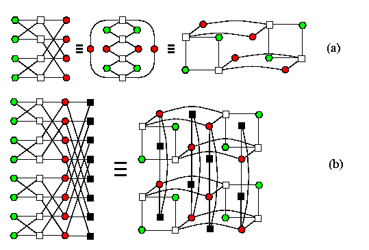
- wBFn can be embedded into CCCn with \dil=\ecng=2.
- The argument is based on vertex symmetry of both topologies and idempotent vertex mapping of each elementary butterfly 2× 2 onto CCC paths consisting of 3 edges: cycle+hypercube+cycle (see Figure). So, CCCn can simulate wBFn with slowdown 2.

CAPTION: The idea of embedding wBFn into CCCn with \dil=\ecng=2 and \load=1. Here, x'=\noni(x).
- oBFn can be embedded into wBFn with \load=2 and \dil=1.
- Just by merging terminal vertices of rows oBFn, we get cycles if wBFn. Hence wBFn can simulate oBFn with slowdown 2.
- wBFn can be embedded into oBFn with constant dilation.
- Proof omitted.
There are other two important results related to hypercubic networks which we will mention here.
Lemma
- an N-node hypercubic network can execute an N-node normal hypercube algorithm with only a constant slowdown
- an N-node butterfly can simulate any bounded-degree N-node network with slowdown O(log N) supposing some preprocessing is allowed.
We will not prove here the first statement. The second statement will be proven in Section 9 of this course.
The class of normal hypercube algorithms comprises a large number of important algorithms, e.g., matrix computations, sorting, collective communication algorithms.
Definition
A hypercube algorithm is said to be normal if only one dimension of hypercube edges is used at any step of the algorithm and if consecutive dimensions are used in consecutive steps.
Embeddings into shuffle-based topologies
Lemma
dB2,n and SEn are computationally equivalent.
Proof
- SEn is a spanning subgraph of dB2,n.
-
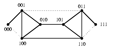
The embedding is again based on one-to-one vertex mapping \varphi:V(SEn)-> V(dB2,n) such that \varphi(u)=\sigma-\parity(u)(u) where \parity is parity is as in Lemma and \sigma is the shuffle operation. Hence, we simply unshuffle all necklaces with vertices with odd parity. Figure shows the undirected case for n=3.

CAPTION: Undirected SE3 is a spanning subgraph of undirected dB2,n.
- dB2,n can be embedded into SEn with \load=1 and \dil=2.
-
the de Bruijn operation of left-shifting accumulates the effects of both shuffle and exchange operations and the argument follows just from using the idempotent vertex mapping.
But there are other interesting structural properties.
Lemma
dB2,n is isomorphic to SEn+1 with contracted exchange arcs.
Proof
If we splice every pair of vertices un... u10 and un... u11 in SEn+1 into vertex un... u1, we get dB2,n.
Lemma
Undirected SEn and dB2,n can simulate n-dimensional normal hypercube algorithms with almost no slowdown.
Proof
Assume a normal hypercube algorithm using consecutively dimensions J=[j1,j2,...]. Two consecutive dimension numbers ji and ji+1 differ by 1 modulo n.
- SEn can simulate a t-step normal Qn algorithm in 2t-1 communication steps.
-
The initial mapping of hypercube nodes onto undirected SEn is such that each node un-1... u0 is mapped to uj1-1... u0 un-1... uj1. Then the first step of the normal hypercube algorithm can be directly simulated, since the nodes who need communicate in Qn are linked by exchange edges in SEn. Assume j2=j1+1. Using the shuffle-edges, we first move every hypercube node un-1... u0 from uj1-1... u0un-1... uj1 to uj1... u0un-1... uj1+1=uj2-1... u0un-1... uj2. In other words, we shuffle all necklaces. Then we can again simulate the hypercube communication along dimension j2 in one step using the exchange arcs in SEn. (If j2=j1-1, we would unshuffle necklaces.) The simulation proceeds in this way for all subsequent steps. So one step of the hypercube algorithm is simulated by two steps of undirected SEn. If the overhead of the initial mapping is ignored, the total number of steps of the simulation is 2t-1.
- dB2,n can simulate a t-step normal Qn algorithm in t communication steps and 2t computational steps.
- It we contract exchange edges into vertices to get dB2,n-1 from SEn, the same vertex mapping enables the same simulation to be performed on undirected dB2,n-1 in t communication steps since the communication along the exchange edges is internal within de Bruijn nodes. Of course, one de Bruijn node simulates two hypercube nodes, so that the local processing is twice of that in the hypercube.
|

