<?xml version="1.0" encoding="utf-8"?><feed xmlns="http://www.w3.org/2005/Atom" ><generator uri="https://jekyllrb.com/" version="3.10.0">Jekyll</generator><link href="https://pages.cs.wisc.edu/~yichen_wang/feed.xml" rel="self" type="application/atom+xml" /><link href="https://pages.cs.wisc.edu/~yichen_wang/" rel="alternate" type="text/html" /><updated>2026-10-30T17:35:26+00:00</updated><id>https://pages.cs.wisc.edu/~yichen_wang/feed.xml</id><title type="html">Yichen Wang</title><subtitle>personal description</subtitle><author><name>Yichen Wang</name><email>yichen.wang@wisc.edu</email></author><entry><title type="html">When Do Learning Curves Follow Power Laws?</title><link href="https://pages.cs.wisc.edu/~yichen_wang/posts/power-laws/" rel="alternate" type="text/html" title="When Do Learning Curves Follow Power Laws?" /><published>2026-09-28T00:00:00+00:00</published><updated>2026-09-28T00:00:00+00:00</updated><id>https://pages.cs.wisc.edu/~yichen_wang/posts/power-laws-have-a-clock</id><content type="html" xml:base="https://pages.cs.wisc.edu/~yichen_wang/posts/power-laws/"><![CDATA[<p class="research-links"><a href="https://arxiv.org/abs/2609.40148">Paper (arXiv)</a> · <a href="https://github.com/yichenblue/spectra-to-schedules-in-pretraining">Code (GitHub)</a> · <a href="/~yichen_wang/posts/power-laws/zh/">中文版</a></p>

<p class="research-lead">We show a sufficient and necessary condition of scaling laws (partially), point out that the scaling laws can be controlled by the intrinsic time and the ratio between the batch size and learning rate, and validate a successful prediction on 300M nano-GPT training. It can be a good example of how a simple model sparks LLM pre-training.</p>

<figure id="fit-and-predict-preview" class="research-result-pair">
  <div class="research-result-pair__panels">
    <a class="research-result-pair__panel" href="/~yichen_wang/images/power-laws-have-a-clock/llm-global-811-fit.png" aria-label="Enlarge the 8-1-1 fit">
      <span class="research-result-pair__title">Fit on 8-1-1</span>
      <img src="/~yichen_wang/images/power-laws-have-a-clock/llm-global-811-fit.png" alt="300M nanoGPT validation loss under the 8-1-1 schedule, with a fitted response model and an inset enlarging the late-training loss drops." width="1584" height="1072" decoding="async" />
    </a>
    <a class="research-result-pair__panel" href="/~yichen_wang/images/power-laws-have-a-clock/llm-global-wsd-prediction.png" aria-label="Enlarge the WSD prediction">
      <span class="research-result-pair__title">Predict WSD without refitting</span>
      <img src="/~yichen_wang/images/power-laws-have-a-clock/llm-global-wsd-prediction.png" alt="300M nanoGPT validation loss under WSD, with a prediction using parameters frozen from the 8-1-1 fit; the inset enlarges the continuation after the shared checkpoint." width="1609" height="1072" decoding="async" />
    </a>
  </div>
  <figcaption><strong>Fit one schedule, predict another.</strong> Validation loss from our 300M nanoGPT experiment, using our joint-schedule surrogate and the fit-then-transfer protocol of <a href="https://arxiv.org/html/2509.19189v4#S6.SS2">Li et al. (2025)</a>. Fit on 8-1-1 (left), then freeze the parameters and predict WSD's continuation without refitting (right). The runs share a training prefix and branch at the dotted line; the insets enlarge the late-training response. Intrinsic time is \(T=\sum_t\eta_t\), with learning rate \(\eta_t\). Select either panel to enlarge.</figcaption>
</figure>

<p>Scaling laws describe how language-model loss changes with model size, training data, and compute. In many experiments, these relationships are well approximated by power laws. They help us estimate the gains from scaling up and choose a model size and token budget within a fixed compute budget.</p>

<figure id="scaling-law-overview" style="display:block;max-width:680px;margin:1.4em auto;">
  <div style="display:grid;grid-template-columns:repeat(auto-fit,minmax(200px,1fr));gap:0;background:#fff;padding:6px;border-radius:4px;">
    <!-- Preserve the original unequal panel boundaries and a shared scale when stacking. -->
    <div style="overflow:hidden;min-width:0;width:100%;max-width:260px;margin:0 auto;">
      <img src="/~yichen_wang/images/power-laws-have-a-clock/kaplan-2020-scaling-laws.svg" alt="Kaplan et al. compute scaling: pale training trajectories and their efficient frontier follow a power-law trend." style="display:block;width:283.201761%;max-width:none;height:auto;margin:0;clip-path:inset(0 64.689485% 0 0);" />
    </div>
    <div style="overflow:hidden;min-width:0;width:100%;max-width:260px;margin:0 auto;">
      <img src="/~yichen_wang/images/power-laws-have-a-clock/kaplan-2020-scaling-laws.svg" alt="Kaplan et al. dataset scaling: test loss decreases regularly as dataset size increases." style="display:block;width:283.201761%;max-width:none;height:auto;margin:0;clip-path:inset(0 31.599757% 0 35.310515%);transform:translateX(-34.200121%);" />
    </div>
    <div style="overflow:hidden;min-width:0;width:100%;max-width:260px;margin:0 auto;">
      <img src="/~yichen_wang/images/power-laws-have-a-clock/kaplan-2020-scaling-laws.svg" alt="Kaplan et al. parameter scaling: test loss follows an approximate power law in non-embedding parameter count." style="display:block;width:283.201761%;max-width:none;height:auto;margin:0;clip-path:inset(0 0 0 68.400243%);transform:translateX(-66.544864%);" />
    </div>
  </div>
  <figcaption><strong>Regular scaling across compute, data, and model size.</strong> <a href="https://arxiv.org/html/2001.08361v1#S1.F1">Kaplan et al. (2020), Figure 1</a>.</figcaption>
</figure>

<p>At a fixed compute budget, a larger model leaves fewer tokens for training. Chinchilla (<a href="https://arxiv.org/html/2203.15556v1#S3.SS3">Hoffmann et al. (2022)</a>) captures this trade-off by fitting a <strong>power-law scaling law</strong> for the final loss of a model with \(N\) parameters trained on \(D\) tokens:</p>

\[L(N,D)\approx L_\infty+\frac{A_N}{N^\alpha}+\frac{A_D}{D^\beta}.\]

<p>Here \(L_\infty\) is the fitted loss floor. The two excess-loss terms decay as power laws: \(N^{-\alpha}\) in model size and \(D^{-\beta}\) in training tokens, with fitted amplitudes \(A_N,A_D\) and exponents \(\alpha,\beta\).</p>

<p>Extending a fitted curve beyond the observed range is easy; knowing when to trust it is harder. Models, data, and training recipes can all change these relationships.</p>

<p>In the synthetic regression experiment of <a href="https://www.opt-ml.org/papers/2024/paper78.pdf#page=6">Qiu et al. (2024)</a>, MLPs learning a target with an exponential frequency distribution produce a compute–loss frontier that is not well described by a power law. The training recipe matters too. In the language-model experiments of <a href="https://arxiv.org/html/2406.19146v4#A9">Porian et al. (2024)</a>, a power law extrapolates well under a tuned recipe, but poorly under other recipes.</p>

<figure id="scaling-frontier-triptych" class="research-frontier-triptych">
  <div class="research-frontier-triptych__scroll" role="region" aria-label="Three compute-frontier panels; scroll horizontally on narrow screens" tabindex="0">
    <div class="research-frontier-triptych__panels">
      <a id="task-dependent-scaling-frontier" class="research-frontier-triptych__panel" href="/~yichen_wang/images/power-laws-have-a-clock/qiu-2024-no-power-law.png" aria-label="View the full-size Qiu Figure 3(c) crop">
        <span class="research-frontier-triptych__title">(a) Synthetic regression</span>
        <svg xmlns="http://www.w3.org/2000/svg" viewBox="0 26 636 479" role="img" aria-label="Qiu Figure 3(c): the synthetic MLP compute–loss frontier departs from the dashed best power-law fit.">
          <image href="/~yichen_wang/images/power-laws-have-a-clock/qiu-2024-no-power-law.png" width="636" height="615" />
        </svg>
      </a>
      <a id="training-dependent-scaling-frontier" class="research-frontier-triptych__panel" href="/~yichen_wang/images/power-laws-have-a-clock/porian-2024-training-recipes.png" aria-label="View the full-size Porian Figure 19 crop">
        <span class="research-frontier-triptych__title">(b) Optimizer tuning (no decay)</span>
        <svg xmlns="http://www.w3.org/2000/svg" viewBox="0 44 580 544" role="img" aria-label="Porian Figure 19, tuned optimizer without decay: higher-compute optimal losses track the power-law extrapolation.">
          <image href="/~yichen_wang/images/power-laws-have-a-clock/porian-2024-training-recipes.png" width="1160" height="598" />
        </svg>
      </a>
      <a class="research-frontier-triptych__panel" href="/~yichen_wang/images/power-laws-have-a-clock/porian-2024-training-recipes.png" aria-label="View the full-size Porian Figure 19 crop">
        <span class="research-frontier-triptych__title">(c) Cosine decay</span>
        <svg xmlns="http://www.w3.org/2000/svg" viewBox="580 44 580 544" role="img" aria-label="Porian Figure 19, cosine decay: higher-compute optimal losses depart from the power-law extrapolation.">
          <image href="/~yichen_wang/images/power-laws-have-a-clock/porian-2024-training-recipes.png" width="1160" height="598" />
        </svg>
      </a>
    </div>
  </div>
  <div class="research-frontier-triptych__hint">Scroll sideways to view all three panels; select a panel to enlarge.</div>
  <figcaption><strong>Power-law fits across tasks and training recipes.</strong> (a) Synthetic MLP regression; dashed line: best power-law fit. Cropped from <a href="https://www.opt-ml.org/papers/2024/paper78.pdf#page=6">Qiu et al. (2024), Figure 3(c)</a>. (b–c) Estimated optimal language-model loss versus compute; open markers: optimal-loss estimates; dashed lines: extrapolation. Cropped from <a href="https://arxiv.org/pdf/2406.19146v4#page=28">Porian et al. (2024), Figure 19</a> (<a href="https://creativecommons.org/licenses/by/4.0/">CC BY 4.0</a>).</figcaption>
</figure>

<p>To understand when these frontiers follow power laws—and when they do not—we first need to understand the individual training curves that make them up: with model and data fixed, when does loss decay as a power law, and how does training change that law?</p>

<p>Within a given training phase, a model’s loss can be fitted as</p>

\[L(t)\approx a\,t^{-p},\]

<p>where \(t\) counts training steps, \(a\) is the fitted amplitude, and \(p\) is the phase’s decay exponent. To see how training affects \(p\), compare runs with different learning-rate schedules.</p>

<p><a href="https://arxiv.org/html/2506.05447v1#A3.SS3">Mircea et al. (2025)</a> compared separate runs with the same architecture, data, and other settings: one used warmup followed by a constant learning rate; the other used warmup followed by cosine decay.</p>

<figure id="learning-rate-scaling-exponents" style="display:block;max-width:620px;margin:1.4em auto;">
  <div style="display:grid;grid-template-columns:repeat(auto-fit,minmax(220px,1fr));gap:16px;background:#fff;padding:8px;border-radius:4px;">
    <div style="min-width:0;text-align:center;">
      <p style="margin:0 0 8px;font-size:0.85em;font-weight:600;">Warmup + constant LR</p>
      <a href="https://arxiv.org/html/2506.05447v1#S2.F2" aria-label="View Figure 2 in Mircea et al.">
        <svg xmlns="http://www.w3.org/2000/svg" viewBox="0 0 300 456" role="img" aria-label="Figure 2: log–log loss curves and broken-power-law fits, with constant learning rate after warmup for the 14M–472M models." style="display:block;width:100%;height:330px;margin:0;">
          <image href="/~yichen_wang/images/power-laws-have-a-clock/mircea-2025-constant-lr.svg" width="278.56315" height="411.96699" transform="translate(13.973956 16.79999)" />
        </svg>
      </a>
    </div>
    <div style="min-width:0;text-align:center;">
      <p style="margin:0 0 8px;font-size:0.85em;font-weight:600;">Warmup + cosine decay</p>
      <a href="https://arxiv.org/html/2506.05447v1#A3.SS3" aria-label="View Figure 29 and the learning-rate comparison in Mircea et al.">
        <svg xmlns="http://www.w3.org/2000/svg" viewBox="0 0 300 456" role="img" aria-label="Figure 29: log–log loss curves and broken-power-law fits with cosine learning-rate decay; the 14M–472M models have steeper fitted late-training slopes." style="display:block;width:100%;height:330px;margin:0;">
          <image href="/~yichen_wang/images/power-laws-have-a-clock/mircea-2025-cosine-lr.svg" width="216" height="360" transform="matrix(1.3333333333333333 0 0 1.25 2.4 1.5)" />
        </svg>
      </a>
    </div>
  </div>
  <figcaption><strong>Changing the schedule changes the fitted exponent.</strong> <a href="https://arxiv.org/html/2506.05447v1#A3.SS3">Mircea et al. (2025), Figures 2 and 29</a>.</figcaption>
</figure>

<p>Compare the 144M model across the two panels: cosine decay raises its fitted late-training exponent from <strong>0.023 to 0.036</strong>. The fitted slope depends on the training schedule, not just the model and dataset.</p>

<p>These examples connect several questions: when loss follows a power law, why power laws arise (<a href="https://arxiv.org/abs/2606.25008">Liu and Gore (2026)</a>), and how data and task structure interact with the training schedule to determine the exponent (<a href="https://arxiv.org/abs/2210.16859">Maloney et al. (2022)</a>). To answer them, we start with the updates of stochastic gradient descent (SGD).</p>

<h2 id="why-sgd-has-memory">SGD has memory</h2>

<p>SGD estimates gradients with minibatches. Compared with full-gradient updates, sampling error randomly perturbs the parameters. Later updates continue from those changed parameters, so a perturbation can affect loss for many steps.</p>

<p>For a model \(f_\theta\) with training objective \(\mathcal L\), let \(\eta_t\) be the learning rate, \(B_t\) the batch size, and \(\xi_t\) the minibatch-gradient error. With fresh i.i.d. examples, SGD takes the form</p>

\[\theta_{t+1}
=\theta_t-\eta_t\nabla\mathcal L(\theta_t)-\eta_t\xi_t,
\qquad
\mathbb E_t[\xi_t]=0,
\qquad
\operatorname{Cov}_t(\xi_t)=\frac{\Sigma(\theta_t)}{B_t}.\]

<p>Here expectations are conditional on the training history, and \(\Sigma\) is the single-example gradient covariance. The parameter perturbation \(-\eta_t\xi_t\) therefore has variance scale \(\eta_t^2/B_t\): a smaller learning rate or a larger batch reduces its size. What matters for a later loss is how subsequent updates propagate that perturbation.</p>

<p>A small-noise expansion lets us add up these effects. Write \(F(n)\) for the noise-free validation loss and \(K(n,s)\) for the response at update \(n\) to noise injected at update \(s\):</p>

\[\mathbb E L_{\mathrm{val}}(\theta_n)
\approx
\underbrace{F(n)}_{\text{baseline learning}}
+\sum_{s&lt;n}
\underbrace{\frac{\eta_s^2}{B_s}}_{\text{injected variance scale}}
\underbrace{K(n,s)}_{\text{effect on the final loss}}.\]

<p>The first term follows full-gradient updates from the same initialization and with the same learning-rate schedule; the sum collects the effects of minibatch noise. This is the starting point of the <strong>forcing–memory decomposition</strong>.</p>

<details>
  <summary><strong>Derivation details: from SGD updates to the memory response</strong></summary>

  <p>Fix a horizon \(n\), an initialization \(\theta_0\), and deterministic schedules \((\eta_t,B_t)\). Let \(\theta_t\in\mathbb R^p\) be the parameters before update \(t\). Each update uses fresh i.i.d. examples from the same data distribution. Assume the smoothness and moment bounds required by the expansions below.</p>

  <p><strong>1. The size of the sampling noise.</strong> For the model \(f_\theta\) and per-example loss \(\ell(f_\theta;z)\), write \(\mathcal L(\theta)=\mathbb E_z[\ell(f_\theta;z)]\) and \(g(\theta;z)=\nabla_\theta\ell(f_\theta;z)\). At update \(t\), let \(z_{t,i}\) be the \(i\)-th example in the batch. The minibatch gradient \(\widehat g_t\) and its sampling error \(\xi_t\) are</p>

\[\widehat g_t=\frac1{B_t}\sum_{i=1}^{B_t}g(\theta_t;z_{t,i}),
\qquad
\xi_t=\widehat g_t-\nabla\mathcal L(\theta_t).\]

  <p>Let \(\mathbb E_t\) denote expectation conditional on the training history, and \(\mathbb E\) expectation over all batches. Define the single-example gradient covariance \(\Sigma(\theta)=\operatorname{Cov}_z(g(\theta;z))\). Conditional independence of the examples gives</p>

\[\mathbb E_t[\xi_t]=0,
\qquad
\mathbb E_t[\xi_t\xi_t^{\!\top}]
=\frac1{B_t^2}\sum_{i=1}^{B_t}\Sigma(\theta_t)
=\frac{\Sigma(\theta_t)}{B_t}.\]

  <p>The parameter perturbation is \(h_t=-\eta_t\xi_t\), so \(\mathbb E_t\lVert h_t\rVert^2=\eta_t^2\operatorname{Tr}\Sigma(\theta_t)/B_t\). This separates the schedule-dependent variance scale, \(\eta_t^2/B_t\), from the state-dependent gradient covariance.</p>

  <p><strong>2. How one perturbation travels through later updates.</strong> Define the full-gradient update map \(D_t\) and its reference trajectory \(\bar\theta_t\):</p>

\[D_t(\theta)=\theta-\eta_t\nabla\mathcal L(\theta),
\qquad
\bar\theta_{t+1}=D_t(\bar\theta_t),
\qquad
\bar\theta_0=\theta_0.\]

  <p>Inject \(h_s=-\eta_s\xi_s\) at a single update \(s\), using full-gradient updates otherwise. Let \(\delta_t^{(s)}\) be the displacement from \(\bar\theta_t\). With a locally Lipschitz Hessian, subtracting the two updates and expanding for \(t\ge s+1\) gives</p>

\[\begin{aligned}
\delta_{t+1}^{(s)}
&amp;=D_t(\bar\theta_t+\delta_t^{(s)})-D_t(\bar\theta_t)\\
&amp;=\left[I-\eta_t\nabla^2\mathcal L(\bar\theta_t)\right]\delta_t^{(s)}
+O\!\left(\eta_t\|\delta_t^{(s)}\|^2\right).
\end{aligned}\]

  <p>Starting from \(\delta_{s+1}^{(s)}=-\eta_s\xi_s\) and retaining the linear term gives</p>

\[\delta_n^{(s)}\approx-\eta_s A_{n-1}\cdots A_{s+1}\xi_s,
\qquad
A_t=I-\eta_t\nabla^2\mathcal L(\bar\theta_t).\]

  <p>Here \(A_t\) is the update Jacobian along the reference trajectory. The product describes how later updates reshape the original perturbation; the empty product is \(I\).</p>

  <p><strong>3. How the perturbation changes the final loss.</strong> Let \(L_{\mathrm{val}}\) be the validation loss. Define \(G_{n,s}(\theta)\) as the final validation loss obtained by starting from \(\theta\) at update \(s\) and following the remaining full-gradient updates:</p>

\[G_{n,s}(\theta)
=L_{\mathrm{val}}\!\left((D_{n-1}\circ\cdots\circ D_s)(\theta)\right),
\qquad
G_{n,n}(\theta)=L_{\mathrm{val}}(\theta).\]

  <p>By construction, \(G_{n,s}=G_{n,s+1}\circ D_s\).</p>

  <p>Write \(\Psi=D_{n-1}\circ\cdots\circ D_{s+1}\) for the map from parameters after update \(s\) to final parameters, with coordinates \(\Psi_i\). Then \(G_{n,s+1}=L_{\mathrm{val}}\circ\Psi\), and the second-order chain rule gives</p>

\[\begin{aligned}
\nabla^2G_{n,s+1}(\theta)
={}&amp;\left[\frac{\partial\Psi}{\partial\theta}(\theta)\right]^{\!\top}
\nabla^2L_{\mathrm{val}}(\Psi(\theta))\,\frac{\partial\Psi}{\partial\theta}(\theta)\\
&amp;+\sum_{i=1}^{p}
\partial_i L_{\mathrm{val}}(\Psi(\theta))\,\nabla^2\Psi_i(\theta).
\end{aligned}\]

  <p>At \(\bar\theta_{s+1}\), the remaining updates end at \(\bar\theta_n\), and \(\frac{\partial\Psi}{\partial\theta}\) equals \(A_{n-1}\cdots A_{s+1}\). Substituting gives</p>

\[\begin{aligned}
\nabla^2G_{n,s+1}(\bar\theta_{s+1})
={}&amp;(A_{n-1}\cdots A_{s+1})^{\!\top}
\nabla^2L_{\mathrm{val}}(\bar\theta_n)
(A_{n-1}\cdots A_{s+1})\\
&amp;+\sum_{i=1}^{p}
\partial_i L_{\mathrm{val}}(\bar\theta_n)\,\nabla^2\Psi_i(\bar\theta_{s+1}).
\end{aligned}\]

  <p>The propagation matrices thus enter the curvature of the future loss. The first term measures how loss responds to the spread in final parameters. The second captures the shift in their mean caused by nonlinear updates: a mean-zero perturbation need not remain mean-zero after nonlinear propagation. Both contribute at second order, so both must be retained.</p>

  <p>Return to the actual SGD trajectory and define \(\theta_s^+=D_s(\theta_s)\), the state after the full-gradient part of update \(s\). Since \(\theta_{s+1}=\theta_s^+ +h_s\), a conditional Taylor expansion gives</p>

\[\begin{aligned}
&amp;\mathbb E_s\!\left[G_{n,s+1}(\theta_s^+ +h_s)-G_{n,s+1}(\theta_s^+)\right]\\
&amp;\quad=\frac12\mathbb E_s\!\left[
h_s^{\!\top}\nabla^2G_{n,s+1}(\theta_s^+)h_s\right]
+O\!\left(\eta_s^3\mathbb E_s\|\xi_s\|^3\right)\\
&amp;\quad=\frac{\eta_s^2}{2B_s}\operatorname{Tr}\!\left[
\Sigma(\theta_s)\nabla^2G_{n,s+1}(\theta_s^+)
\right]
+O\!\left(\eta_s^3\mathbb E_s\|\xi_s\|^3\right).
\end{aligned}\]

  <p>The linear term vanishes because \(\mathbb E_s[h_s]=0\), and the second equality uses \(\mathbb E_s[h_sh_s^{\top}]=\eta_s^2\Sigma(\theta_s)/B_s\). The higher-order remainder is controlled by third derivatives of the future loss along the segment from \(\theta_s^+\) to \(\theta_s^+ +h_s\).</p>

  <p><strong>4. Adding the effects of all updates.</strong> A telescoping sum cancels the intermediate future-loss values, leaving the difference between the final SGD loss and the noise-free baseline:</p>

\[\begin{aligned}
L_{\mathrm{val}}(\theta_n)-G_{n,0}(\theta_0)
&amp;=\sum_{s&lt;n}\left[G_{n,s+1}(\theta_{s+1})-G_{n,s}(\theta_s)\right]\\
&amp;=\sum_{s&lt;n}\left[
G_{n,s+1}(\theta_s^+ +h_s)-G_{n,s+1}(\theta_s^+)
\right].
\end{aligned}\]

  <p>Taking expectations, define the noise-free baseline \(F(n)=G_{n,0}(\theta_0)\) and the response coefficient</p>

\[K(n,s)
:=\frac12\mathbb E\!\left[
\operatorname{Tr}\!\left(
\Sigma(\theta_s)\nabla^2G_{n,s+1}(D_s(\theta_s))
\right)\right].\]

  <p>Let \(\mathcal E_n\) collect the expected higher-order remainders over all updates. Inserting the expansion from step 3 gives</p>

\[\mathbb E L_{\mathrm{val}}(\theta_n)
=F(n)
+\sum_{s&lt;n}\frac{\eta_s^2}{B_s}K(n,s)
+\mathcal E_n.\]

  <p>Earlier noise has not been removed from this calculation: \(\theta_s\) already depends on all preceding batches. The average defining \(K(n,s)\) therefore includes how earlier noise changes the state reached at update \(s\).</p>

  <p><strong>5. The error left by the approximation.</strong> Let \(M_{n,s}\) uniformly bound \(|\nabla^3G_{n,s+1}|\) along the Taylor segments, over the sampled histories under consideration. Then</p>

\[|\mathcal E_n|
\le\frac16\sum_{s&lt;n}
M_{n,s}\eta_s^3\mathbb E\|\xi_s\|^3.\]

  <p>Omitting \(\mathcal E_n\) gives the response approximation in the main text. At fixed horizon, scaling the sampling noise by \(\epsilon\) makes the retained contribution quadratic in \(\epsilon\) to leading order, while the remainder is \(O(\epsilon^3)\), under uniform derivative and third-moment bounds.</p>

  <p>The calculation tells us what \(K(n,s)\) measures: how noise added at update \(s\) affects loss at update \(n\), including the effects of the states reached during training. Describing how that response changes over time by a power law with a positive decay exponent requires further modeling. The next sections explain how the spectral model produces such a law and how the LLM experiments test whether it predicts loss under a new schedule.</p>

</details>

<p>In our Gaussian random feature model, the features are fixed, the output weights are trainable, and the loss is squared error. SGD’s expected squared prediction error relative to the noise-free target, \(R_t\), obeys the exact recurrence</p>

\[R_t=F_t+\sum_{s&lt;t}K_{t,s}\bigl(R_s+\sigma^2\bigr).\]

<p>\(F_t\) describes how the initial error propagates, while the history sum describes the accumulated effects of training noise. The remaining prediction error \(R_s\) at step \(s\) and the label-noise variance \(\sigma^2\) both contribute to the noise, and \(K_{t,s}\) describes its effect on loss at step \(t\).</p>

<p><strong>Bias–variance gives another grouping of the same dynamics.</strong> Consider a target the model can represent, and assume label noise is independent of the input and has mean zero. Following the decomposition by error source in <a href="https://arxiv.org/html/2103.12692v3#S4.SS2">Zou et al. (2021)</a>, write \(B_t\) for the error from clean-label SGD and \(V_t\) for the error driven by label noise from zero initial error. Only in this comparison, \(B_t\) denotes bias rather than batch size. At every step,</p>

\[\begin{aligned}
R_t
&amp;=\underbrace{F_t+\sum_{s&lt;t}K_{t,s}B_s}_{\text{source bias }B_t}
+\underbrace{\sum_{s&lt;t}K_{t,s}(V_s+\sigma^2)}_{\text{source variance }V_t}\\[6pt]
&amp;=\underbrace{F_t}_{\text{forcing}}
+\underbrace{\sum_{s&lt;t}K_{t,s}(B_s+V_s+\sigma^2)}_{\text{memory}}.
\end{aligned}\]

<p>The first line separates error sources: the initial error and its sampling effects, or label noise and its subsequent effects. The second separates forcing from the accumulated effects of history. In particular, \(\sum_{s&lt;t}K_{t,s}B_s\) belongs to bias in the first line and memory in the second. Clean labels make \(V_t=0\), but do not remove this part of the memory term. The two decompositions group the same effects differently; memory is not the same as label-noise variance.</p>

<details>
  <summary><strong>Derivation details: from the Volterra equation to the bias–variance decomposition</strong></summary>

  <p>Use the Gaussian random feature model, realizable target, and label-noise assumptions from the main text, fixing the features, input distribution, and predetermined learning-rate and batch-size schedules. Here \(K_{t,s}\) does not depend on the initial error or label-noise variance, so the following two processes use the same kernel.</p>

  <p><strong>1. Remove label noise and retain minibatch sampling.</strong> Keep the original initialization and set \(\sigma^2=0\). The Volterra equation gives the error of clean-label SGD:</p>

\[B_t=F_t+\sum_{s&lt;t}K_{t,s}B_s.\]

  <p>Source bias therefore includes the sampling effects of clean-label training as well as \(F_t\).</p>

  <p><strong>2. Remove the initial error and retain label noise.</strong> Starting from zero initial prediction error makes the forcing term zero, giving</p>

\[V_t=\sum_{s&lt;t}K_{t,s}(V_s+\sigma^2).\]

  <p>Zero initial error means that the model already makes the correct noise-free predictions at the start of training; it does not mean initializing the parameters to zero. This process isolates label noise and its subsequent effects.</p>

  <p><strong>3. Add the two recurrences.</strong> This gives</p>

\[B_t+V_t
=F_t+\sum_{s&lt;t}K_{t,s}(B_s+V_s+\sigma^2).\]

  <p>This is the same recurrence as for \(R_t\). Since \(B_0=R_0\), \(V_0=0\), and each step depends only on earlier times, induction gives \(R_t=B_t+V_t\). Substituting the expression for \(B_t\) yields the two groupings in the main text.</p>

</details>

<p>These decompositions identify the effects that contribute to loss, but do not yet explain how they decay over time. To understand where power laws come from, we need to look at how quickly error fades in each direction.</p>

<h2 id="different-directions-learn-at-different-speeds">Different directions learn at different speeds</h2>

<p>Continue with the model \(f_a(x)=a^\top\phi(x)\), with fixed features \(\phi\) and trainable weights \(a\). We can explicitly calculate how quickly errors fade in each direction, as in the compute-optimal scaling analysis of <a href="https://proceedings.neurips.cc/paper_files/paper/2024/hash/1dccfc3ee01871d05e33457c61037d59-Abstract-Conference.html">Paquette et al. (2024)</a>.</p>

<p>These differences in speed are visible in the loss landscape: its curvature can vary across Hessian eigenvector directions. The left panel below sketches a quadratic loss, with a steep blue direction and a flatter orange direction.</p>

<figure id="fast-slow-landscape">
  <a href="/~yichen_wang/images/power-laws-have-a-clock/fast-slow-landscape.png" aria-label="Enlarge the landscape illustration of fast and slow directions">
    <img src="/~yichen_wang/images/power-laws-have-a-clock/fast-slow-landscape.png" alt="Left: a steep blue cross-section and a flatter orange cross-section of the same quadratic loss landscape. Right: the two directions at the same scale, starting from the same parameter error and taking four full-gradient updates at the same learning rate. The error shrinks much more in the blue direction than in the orange direction." width="2271" height="1091" loading="lazy" decoding="async" style="display:block;width:100%;height:auto;" />
  </a>
</figure>

<p>The right panel places both cross-sections on the same axes: parameter error horizontally and the direction’s contribution to loss vertically. The two open circles mark initial parameter errors of the same size. After four full-gradient updates at the same learning rate, the error in the blue direction has shrunk substantially, while the error in the orange direction has fallen only slightly.</p>

<p>To see why, write the parameter error in direction \(j\) as \(\rho_j\) and its Hessian eigenvalue as \(\lambda_j\). Its loss contribution is \(\frac12\lambda_j\rho_j^2\), and its gradient component is \(\lambda_j\rho_j\). For the same parameter error, a larger positive eigenvalue means a steeper landscape and a larger gradient. At the same sufficiently small learning rate, each update therefore removes a larger fraction of the error. We call directions where errors fade quickly “fast directions,” and those where errors fade slowly “slow directions.”</p>

<p>Let \(\rho_{j,t}\) denote the parameter error in this direction at step \(t\). Repeated full-gradient updates give, under the small-step approximation,</p>

\[\rho_{j,t}\approx\rho_{j,0}e^{-\lambda_jT_t},
\qquad
T_t=\sum_{s&lt;t}\eta_s.\]

<p>The clock \(T_t\) is <strong>intrinsic time</strong>. Reducing a direction’s error by a fixed factor takes intrinsic time proportional to \(1/\lambda_j\).</p>

<p>Loss adds up weighted squared errors across directions. A slow direction contributes little if there was almost no error there to begin with. Learning speed and importance to the loss are different things.</p>

<details>
  <summary><strong>Derivation details: from squared loss to learning time</strong></summary>

  <p><strong>1. From squared loss to the gradient.</strong> Let \(\phi(x)\) be the fixed feature vector for input \(x\), \(y\) its target, and \(a\) the trainable weights. Define the population squared loss and its Hessian:</p>

\[\mathcal L(a)=\frac12\mathbb E\!\left[(a^\top\phi(x)-y)^2\right],
\qquad
H=\mathbb E[\phi(x)\phi(x)^\top].\]

  <p>For a minimizer \(a_\star\), the condition \(\nabla\mathcal L(a_\star)=0\) gives \(\mathbb E[\phi(x)y]=Ha_\star\). Hence</p>

\[\nabla\mathcal L(a)
=\mathbb E\!\left[\phi(x)(a^\top\phi(x)-y)\right]
=H(a-a_\star).\]

  <p>The gradient is the remaining parameter error transformed by \(H\). This identity is exact for squared loss with fixed features.</p>

  <p><strong>2. From the gradient to error dynamics.</strong> First consider full-gradient training, without batch-sampling noise. With learning rate \(\eta_t\) and parameter error \(e_t=a_t-a_\star\), the update becomes</p>

\[\begin{aligned}
a_{t+1}&amp;=a_t-\eta_t\nabla\mathcal L(a_t),\\
e_{t+1}&amp;=e_t-\eta_tHe_t=(I-\eta_tH)e_t.
\end{aligned}\]

  <p>Let \((\lambda_j,u_j)\) be an orthonormal eigensystem of the symmetric matrix \(H\), and define \(\rho_{j,t}=u_j^\top e_t\). Projecting the update onto \(u_j\) gives</p>

\[\begin{aligned}
\rho_{j,t+1}
&amp;=u_j^\top(I-\eta_tH)e_t\\
&amp;=(1-\eta_t\lambda_j)\rho_{j,t},
\qquad Hu_j=\lambda_j u_j.
\end{aligned}\]

  <p>Along direction \(u_j\), the gradient is \(\lambda_j\) times the remaining error. In the small-step regime, one update therefore removes a fraction \(\eta_t\lambda_j\) of that error.</p>

  <p><strong>3. From the recurrence to a learning time scale.</strong> Iterating from the initial error \(\rho_{j,0}\) gives</p>

\[\rho_{j,t}
=\rho_{j,0}\prod_{s&lt;t}(1-\eta_s\lambda_j).\]

  <p>For \(\eta_s\lambda_j\ll1\), using \(\log(1-x)\approx-x\) yields the intrinsic-time approximation</p>

\[\rho_{j,t}\approx\rho_{j,0}e^{-\lambda_jT_t},
\qquad
T_t=\sum_{s&lt;t}\eta_s.\]

  <p>For \(\lambda_j&gt;0\), let \(T_{\mathrm{learn},j}\) denote the intrinsic time needed to reduce the error magnitude by a fixed factor, and \(t_{\mathrm{learn},j}\) the corresponding number of updates. At constant learning rate \(\eta\),</p>

\[T_{\mathrm{learn},j}\asymp\frac1{\lambda_j},
\qquad
t_{\mathrm{learn},j}\asymp\frac1{\eta\lambda_j}.\]

  <p>Large eigenvalues mean short learning times; small eigenvalues mean persistent errors. At time \(T\), modes with \(\lambda_jT\gg1\) have largely decayed, while those with \(\lambda_jT\ll1\) remain close to their initial values.</p>

  <p><strong>4. From directional errors to loss.</strong> The excess squared loss is</p>

\[\begin{aligned}
\mathcal L(a_t)-\mathcal L(a_\star)
&amp;=\frac12e_t^\top He_t
=\frac12\sum_j\lambda_j\rho_{j,t}^2\\
&amp;\approx\frac12\sum_j\lambda_j\rho_{j,0}^2e^{-2\lambda_jT_t}.
\end{aligned}\]

  <p>The eigenvalues set the decay speeds, while the initial error in each direction sets its weight in the loss. This is why knowing the eigenvalues alone is not enough: we also need to know which directions matter for the target. Batch sampling adds new errors during SGD; the full-gradient calculation above isolates how existing errors decay.</p>

</details>

<h2 id="when-do-these-learning-speeds-produce-a-power-law">When do these learning speeds produce a power law?</h2>

<p>Under a constant, stable schedule, each direction’s contribution decays approximately as \(e^{-2\lambda T}\). By time \(T\), contributions from large-eigenvalue directions have faded substantially, so the remaining response depends mainly on the cumulative weight of eigenvalues near and below \(1/T\).</p>

<p>In our random-feature model, we can write these cumulative weights explicitly for forcing and the response to a single noise injection. The fixed features are \(\phi(x)=W^\top x\), the noiseless target is \(x^\top\theta^\star\), and the input covariance is \(\Lambda\). Let \(\widehat\lambda_j,\widehat u_j\) be the eigenvalues and unit eigenvectors of \(\Lambda^{1/2}WW^\top\Lambda^{1/2}\). Starting from zero output weights, the two cumulative weights are</p>

\[\begin{aligned}
\nu_W^{\mathcal F}((0,x])
&amp;=\sum_{0&lt;\widehat\lambda_j\le x}
\left|\left\langle\widehat u_j,\Lambda^{1/2}\theta^\star\right\rangle\right|^2,\\
\nu_W^{\mathcal K}((0,x])
&amp;=\sum_{0&lt;\widehat\lambda_j\le x}\widehat\lambda_j^2.
\end{aligned}\]

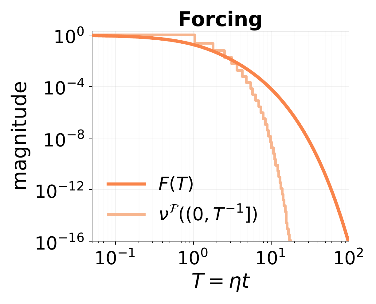
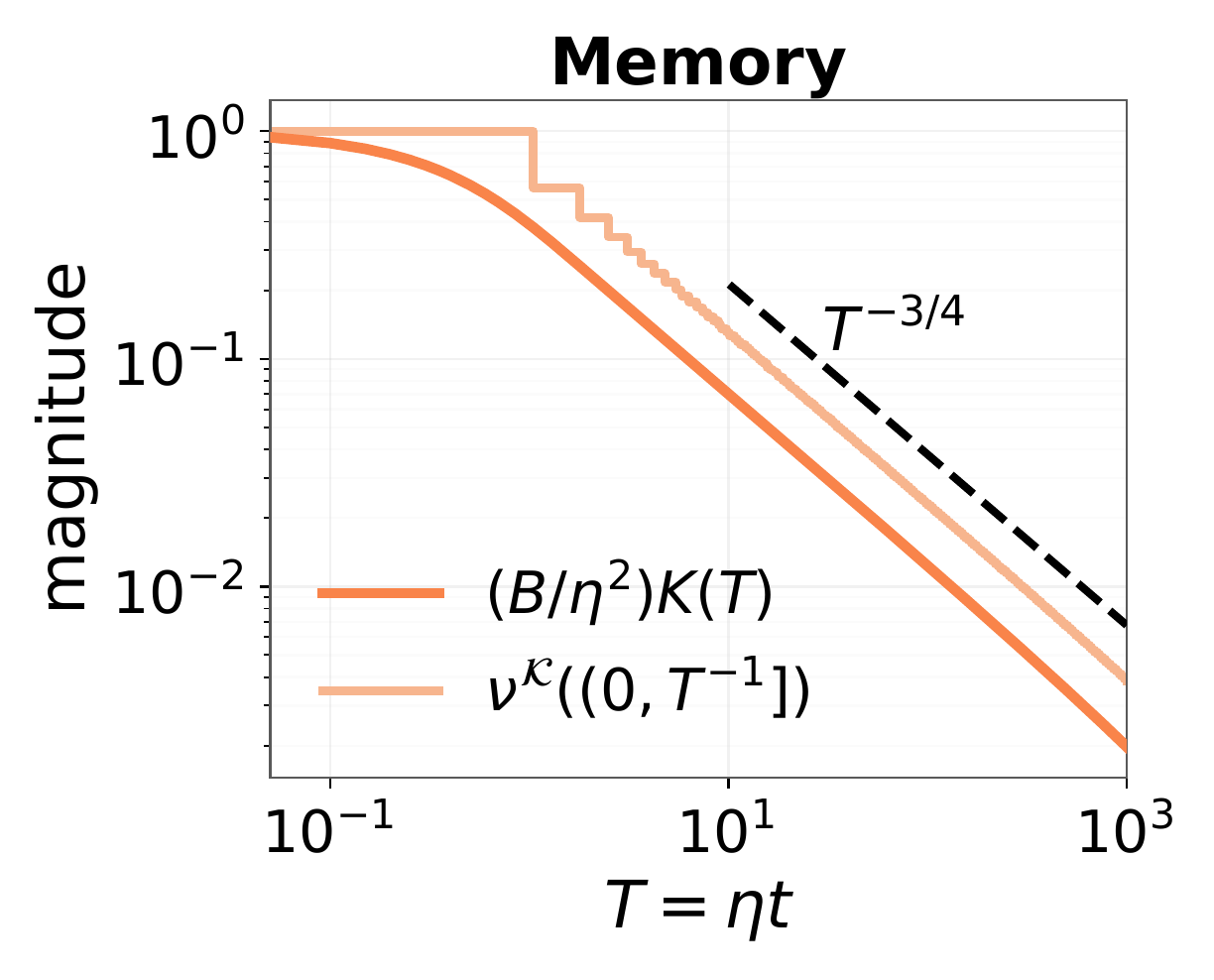
<p>The first line adds up the target energy in these directions; the second adds up the weights of a single-injection memory response. When these totals follow power laws near small eigenvalues, denote their positive exponents by \(q_{\mathcal F}\) and \(q_{\mathcal K}\), respectively.</p>

<p>Our theory shows that, in the paper’s large-width, long-time limit and under its spectral-window conditions, forcing and the single-injection memory response decay as power laws if and only if their respective cumulative spectral weights have the corresponding power-law forms. Schematically,</p>

\[\begin{aligned}
\nu_W^{\mathcal F}((0,x])\propto x^{q_{\mathcal F}}
&amp;\quad\Longleftrightarrow\quad
F_{W,&gt;0}(T)\propto T^{-q_{\mathcal F}},\\
\nu_W^{\mathcal K}((0,x])\propto x^{q_{\mathcal K}}
&amp;\quad\Longleftrightarrow\quad
\frac{B}{\eta^2}K_W(T)\propto T^{-q_{\mathcal K}}.
\end{aligned}\]

<p>Here \(F_{W,&gt;0}\) is the part of forcing above the loss floor, and \(K_W\) is the single-injection memory kernel under a constant schedule. Multiplying by \(B/\eta^2\) removes the noise-injection scale. For the single-injection memory response, \(T\) is the intrinsic time elapsed since injection.</p>

<p>The intuition is that cumulative weight varies as a power of the threshold, while training lowers that threshold to roughly \(1/T\). The same exponent then appears in the decay over time. For a finite model, this power law can hold over a long intermediate time window without continuing indefinitely.</p>

<p>The three panels below use the spectrum</p>

\[\lambda_j=j^{-0.8}.\]

<p>They also use rapidly decaying target coefficients, \(\lvert\theta_j^\star\rvert^2=e^{-j}\). Directions with smaller eigenvalues therefore carry less of the target. Errors fade slowly in those directions, but there is almost no initial signal to learn there; minibatch sampling can still introduce errors.</p>

<figure>
  <div style="display:grid;grid-template-columns:repeat(auto-fit,minmax(220px,1fr));gap:1rem;align-items:end;">
    <img src="/~yichen_wang/images/power-laws-have-a-clock/main-fig2-forcing.png" alt="Target-weighted forcing decaying faster than every inverse power." />
    <img src="/~yichen_wang/images/power-laws-have-a-clock/main-fig2-memory.png" alt="The memory of a single noise injection following a three-quarter power-law tail." />
    <img src="/~yichen_wang/images/power-laws-have-a-clock/main-fig2-loss.png" alt="Small-batch SGD risk crossing into the memory-controlled power-law tail." />
  </div>
  <figcaption><strong>Fast forcing decay, slow memory tail.</strong> Left: forcing vanishes faster than every inverse power. Middle: the memory of a single noise injection decays as \(T^{-3/4}\). Right: SGD loss, averaged over 20 runs, eventually follows that memory tail.</figcaption>
</figure>

<p>The right panel shows how these two contributions shape actual SGD loss: the early decline largely follows forcing, before entering a power-law regime controlled by the history of sampling noise. <strong>The same eigenvalues do not require forcing and memory to follow the same decay law.</strong></p>

<p class="research-takeaway" id="loss-slope-takeaway">A power-law exponent tells us how quickly loss falls, but cannot by itself tell us where the remaining error comes from. Both slowly fading initial error and the lasting effects of training noise can produce power-law tails. Interpreting a learning curve requires separating these contributions, beyond fitting the exponent of their sum.</p>

<p>The equivalences above apply separately to forcing and the single-injection memory response; they do not directly give the exponent of total loss. Recovering the full SGD loss curve also requires accumulating the effects of successive noise injections.</p>

<h2 id="three-kinds-of-memory">Three kinds of memory</h2>

<p>In intrinsic time, write \(k(v)\) for the normalized memory response after a delay \(v\): for the constant reference schedule, \(k(T)=(B/\eta^2)K_W(T)\). The noise-injection strength is supplied separately. To isolate the response itself, first consider a reference setting with the same noise strength injected per unit of intrinsic time. If \(k(v)\asymp(1+v)^{-q_{\mathcal K}}\), the accumulated effects of these injections by time \(T\) have order</p>

\[\int_0^T k(v)\,\mathrm dv
\asymp
\begin{cases}
T^{1-q_{\mathcal K}}, &amp; 0&lt;q_{\mathcal K}&lt;1 \quad(\mathrm{LM}),\\
\log T, &amp; q_{\mathcal K}=1,\\
1, &amp; q_{\mathcal K}&gt;1 \quad(\mathrm{IM}).
\end{cases}\]

<ul>
  <li><strong>Long memory (LM):</strong> Each response fades, but too slowly for the accumulated response to settle under continuing injections. The previous section’s \(q_{\mathcal K}=3/4\) belongs here: equally strong injections yield an accumulated response that grows as \(T^{1/4}\).</li>
  <li><strong>Integrable memory (IM):</strong> Each response fades fast enough for the accumulated response to approach a finite value even as injections continue.</li>
</ul>

<p>At the boundary \(q_{\mathcal K}=1\), the accumulated response grows logarithmically.</p>

<p>To compare responses across different data and targets, now let the target coefficients decay as a power law too:</p>

\[\lambda_j=j^{-2\alpha},
\qquad
|\theta_j^\star|=j^{-\beta}.\]

<p>Here \(\lambda_j\) are ordered data-covariance eigenvalues and \(\theta_j^\star\) the corresponding target coefficients. Larger \(\alpha\) steepens the spectrum; larger \(\beta\) reduces target weight in slow directions.</p>

<p>In the LM/IM region with finite target energy, the cumulative spectral-weight criterion from the previous section gives the exponents of target-dependent forcing and the single-injection memory response:</p>

\[q_{\mathcal F}=\frac{2\alpha+2\beta-1}{2\alpha},
\qquad
q_{\mathcal K}=2-\frac{1}{2\alpha}.\]

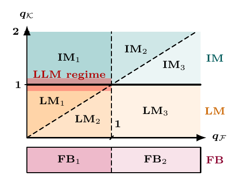
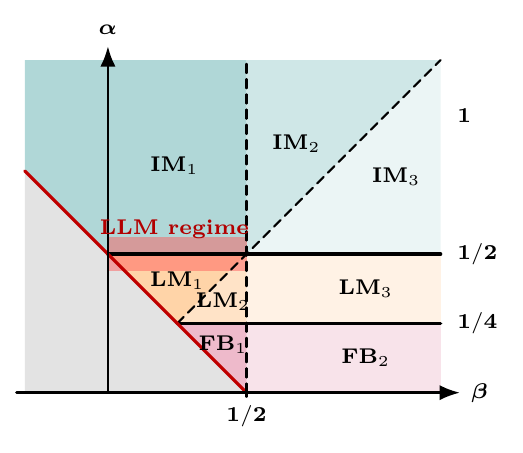
<p>When the spectrum decays more slowly, with \(0&lt;\alpha&lt;1/4\), the single-injection memory weights \(\lambda_j^2\), summed over the many small-eigenvalue directions, still grow with model width. Width then affects the memory response itself, as well as when a power law ends. This is <strong>finite bulk (FB)</strong>: a width-independent positive decay exponent alone cannot describe it.</p>

<p>The two phase diagrams below show these regions in response exponents and in spectrum and target parameters.</p>

<figure class="research-figure--phases" style="display:block;">
  <div style="display:grid;grid-template-columns:minmax(0,1.15fr) minmax(0,1fr);gap:clamp(12px,2vw,24px);align-items:center;width:100%;max-width:680px;margin:0 auto 1rem;">
    <img src="/~yichen_wang/images/power-laws-have-a-clock/main-fig1-response-map.png" alt="Long-memory, integrable-memory, and finite-bulk regimes in forcing–memory response coordinates." style="display:block;width:100%;height:auto;margin:0;" />
    <img src="/~yichen_wang/images/power-laws-have-a-clock/main-fig3-plrf-map.png" alt="The corresponding propagation regimes in the spectrum and target parameters of a power-law random-feature model." style="display:block;width:100%;height:auto;margin:0;" />
  </div>
  <figcaption><strong>Memory regimes in two coordinate systems.</strong> Left: response exponents. Right: spectrum and target parameters, with FB shown separately. The red band marks LLM fits near the LM/IM boundary, \(q_{\mathcal K}=1\).</figcaption>
</figure>

<p>Start with the solid horizontal line in the left panel: it separates LM from IM at \(q_{\mathcal K}=1\), matching the two behaviors of the integral above. In the right panel, this boundary corresponds to a spectral decay rate of \(\alpha=1/2\); FB occupies the separate region \(\alpha&lt;1/4\).</p>

<p>The finer regions compare how quickly target-dependent forcing and memory decay, and whether the former has a finite time integral. In the left panel, the diagonal dashed line marks \(q_{\mathcal F}=q_{\mathcal K}\), and the vertical dashed line marks \(q_{\mathcal F}=1\).</p>

<p>We have now distinguished how the effects of noise fade and accumulate. Actual training also changes the strength of each injection, which is precisely what learning-rate and batch-size schedules can control.</p>

<h2 id="how-training-schedules-transform-the-response">How training schedules transform the response</h2>

<p>Changing the strength of noise injection can directly change the shape of a loss curve. Learning-rate decay offers a familiar example: once the learning rate starts to fall, loss may fall faster. In warmup–stable–decay (WSD) training (<a href="https://arxiv.org/abs/2404.06395">Hu et al. (2024)</a>), the learning rate stays constant after warmup until a final decay phase. Follow the gray-green curves in the MiniCPM experiment below: their gradual decline gives way to a sharp drop when decay begins. The same pattern appears at several different stages of training.</p>

<figure style="display:block;max-width:680px;margin:2em auto;">
  <img src="/~yichen_wang/images/power-laws-have-a-clock/hu-2024-minicpm-wsd-loss.svg" alt="Loss on C4 versus training tokens for a 0.036B model: gray-green WSD curves show sharp drops during decay at several training stages; the orange curve uses cosine decay." style="display:block;width:100%;height:auto;margin:0 auto 1rem;" />
  <figcaption><strong>A sharp loss drop at different stages of training.</strong> The gray-green curves use WSD with different decay timings and durations; orange shows cosine decay. Token counts are expressed as multiples of the model's parameter count, \(N\). Figure reproduced unchanged from the MiniCPM paper, <a href="https://arxiv.org/html/2404.06395v3#S4.F6.fig1">Hu et al. (2024), Figure 5</a>, under <a href="https://creativecommons.org/licenses/by/4.0/">CC BY 4.0</a>.</figcaption>
</figure>

<p>Why does taking smaller updates make loss fall faster? These downward turns look as though the model has begun to learn faster, but reducing the error caused by stochastic updates also lowers loss. If annealing helps, why can’t a more aggressive schedule keep making loss fall faster?</p>

<p>To separate the two effects, start with plain SGD and return to intrinsic time. Lowering the learning rate both shortens the full-gradient update and reduces its noise; increasing batch size reduces noise without shortening that update. The relevant clock and batch-to-learning-rate ratio are</p>

\[T_t=\sum_{s&lt;t}\eta_s,
\qquad
r_t=\frac{B_t}{\eta_t}.\]

<p>An update advances the clock by \(\eta_t\) and injects variance at scale \(\eta_t^2/B_t\). Dividing by the time elapsed in that update gives the noise scale per unit of intrinsic time:</p>

\[\frac{\eta_t^2/B_t}{\eta_t}
=\frac{\eta_t}{B_t}
=\frac{1}{r_t}.\]

<p>\(T_t\) records how far the deterministic learning process described earlier has advanced, while \(1/r_t\) describes the noise scale per unit of progress. Writing \(r(T)\) for the ratio along this clock lets us separate the two effects.</p>

<p>Smaller updates can still make loss fall faster for a while because existing errors fade while new noise keeps adding error. At fixed batch size, lowering the learning rate advances intrinsic time less per update, but also reduces the noise that offsets the decline in loss. If the benefit of noise reduction outweighs the cost of slower progress, loss can drop sharply. This offers one explanation for the WSD curves above, without implying that the model is learning the signal faster.</p>

<p>This separation also appears in the functional scaling law (FSL) of <a href="https://arxiv.org/html/2509.19189v4#S3">Li et al. (2025)</a>: their kernel-regression theory uses intrinsic time to describe learning progress, the learning-rate-to-batch-size ratio to control noise injection, and a forgetting kernel to track its later effects on loss.</p>

<p>This connects increasing batch size with decaying learning rate (<a href="https://arxiv.org/abs/1711.00489">Smith et al. (2018)</a>): both reduce noise per unit of intrinsic time. Since earlier noise can still affect loss, we must match the whole ratio path, not just its final value.</p>

<p>The previous section added up individual responses. Now the noise generated at different times varies in strength: we still add up its surviving effects at the endpoint, but weight each injection by its strength at the time. Returning to the power-law random-feature model, under stable LM/IM schedules and accounting for noise feedback, prediction risk obeys the scaling relation</p>

\[R(T)\asymp
F(T)+
\int_0^T
\frac{F(u)+\sigma^2}{r(u)}
\,k(T-u)\,\mathrm du.\]

<p>Here \(R\) is prediction risk, and \(F\) is the forcing term in the random-feature model, including the loss floor due to finite width; \(\asymp\) allows multiplicative constants.</p>

<p>For a past time \(u\), \(F(u)+\sigma^2\) represents the noise sources supplied by remaining prediction error and label noise in this scaling relation. Dividing by \(r(u)\) lets the schedule adjust the injection strength per unit of intrinsic time; multiplying by \(k(T-u)\) gives its contribution at the endpoint \(T\). Even without label noise, remaining prediction error still generates minibatch noise, so the integral does not vanish when \(\sigma^2=0\).</p>

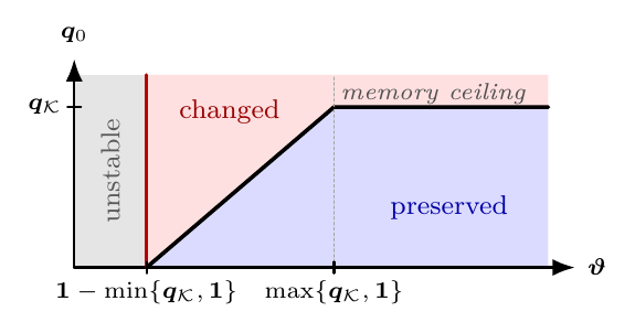
<p>Label noise adds loss relative to clean-label SGD under the same schedule. Within the power-law range above, even if later injections become very small, early noise still leaves a tail that decays as \(k(T)\sim T^{-q_{\mathcal K}}\). The decay exponent of the extra loss therefore cannot exceed \(q_{\mathcal K}\). This is the <strong>memory ceiling</strong>.</p>

<p>More aggressive annealing does not guarantee ever-faster loss decay, for two reasons. First, suppressing new noise does not immediately remove earlier noise: the memory ceiling above limits the power-law exponent of this extra loss in intrinsic time, not the short-term rate of decline per token in the figure. Second, lowering the learning rate more aggressively also slows the clock. At fixed batch size and token budget, less intrinsic time accumulates, leaving less progress in both signal learning and the decay of earlier errors. Annealing can therefore reduce new errors, but it cannot bypass the decay of old ones; pushing it too far can slow that decay down.</p>

<p>When both the individual memory response and ratio growth follow power laws, comparing the extra loss with the excess loss of clean-label SGD gives three outcomes:</p>

<ul>
  <li><strong>Destroy:</strong> the extra loss does not decay as a positive power.</li>
  <li><strong>Change:</strong> the extra loss decays more slowly than the excess loss of clean-label SGD and sets a new exponent.</li>
  <li><strong>Preserve:</strong> the extra loss decays at least as fast, leaving the clean-label SGD exponent unchanged.</li>
</ul>

<p>The diagram compares the clean-label SGD excess-loss exponent \(q_0\), describing decay above its floor as \(T^{-q_0}\), with the ratio-growth exponent \(\vartheta\), defined by \(r(T)\sim T^\vartheta\). Clean-label SGD still includes minibatch noise, so \(q_0\) generally differs from the forcing exponent \(q_{\mathcal F}\).</p>

<figure>
  <img src="/~yichen_wang/images/power-laws-have-a-clock/main-fig4-schedule-map.png" alt="Phase diagram showing when a schedule preserves, changes, or destroys the power law of clean-label SGD." style="display:block;width:min(100%,570px);height:auto;margin-inline:auto;" />
  <figcaption><strong>Preserve, change, or destroy.</strong> Horizontal axis: ratio growth. Vertical axis: clean-label SGD excess-loss decay. The horizontal boundary marks the memory ceiling; \(q_{\mathcal K}=1\) introduces logarithmic corrections.</figcaption>
</figure>

<p>Fix \(q_0\) and move horizontally to the right, increasing \(\vartheta\). If \(q_0&lt;q_{\mathcal K}\), we eventually cross from <strong>change</strong> into <strong>preserve</strong>: the extra loss now decays at least as fast as the excess loss of clean-label SGD. If \(q_0&gt;q_{\mathcal K}\), our horizontal line stays above the memory ceiling, no matter how far right we go. The extra loss has a decay exponent capped at \(q_{\mathcal K}\), so more aggressive noise suppression cannot recover the clean-label SGD exponent.</p>

<h2 id="from-theory-to-llm-pretraining">From theory to LLM pretraining</h2>

<p>The analysis above separated two effects of a schedule: intrinsic time records how far learning has progressed, and \(r(T)\) controls noise injection along the way. Are these quantities still useful for an LLM whose representations keep changing? We first compare different implementations of the same ratio path, then test whether changing that path lets us predict a new loss curve.</p>

<h3 id="two-implementations-of-the-same-ratio-path">Two implementations of the same ratio path</h3>

<p>We first compare two implementations of the same ratio path: we lower the learning rate at fixed batch size in one run and increase the batch size at fixed learning rate in another. We match their clocks and ratio paths.</p>

<p>We made this comparison with a 300M LLM trained using plain SGD on 6.5B OpenWebText tokens. All runs share the first 80% of the token budget, then branch from the same checkpoint for the remaining 20%. In the fixed-batch runs, WSD lowers the learning rate gradually over that tail, while 8-1-1 uses two lower-rate stages of 10% each. If intrinsic time and the ratio path capture the main schedule effects, each learning-rate/batch-size pair should follow nearly the same loss curve.</p>

<figure id="training-clock-animation" style="display:block;">
  <picture>
    <source media="(prefers-reduced-motion: reduce)" srcset="/~yichen_wang/images/power-laws-have-a-clock/main-fig1-clock-animation-still.png" />
    <img src="/~yichen_wang/images/power-laws-have-a-clock/main-fig1-clock-animation.gif" alt="Matched learning-rate and batch-size validation trajectories change from optimizer step to intrinsic time, followed by the 8-1-1 fit, WSD prediction with all parameters fixed, and separation into three layers." width="1100" height="740" loading="lazy" decoding="async" style="display:block;width:100%;height:auto;margin:0;" />
  </picture>
  <figcaption><strong>Different step counts, nearly the same intrinsic-time curves.</strong> The animation switches from optimizer step to \(T=\sum_t\eta_t\), draws the 8-1-1 fit and WSD prediction with all parameters fixed, then unfolds the curves into three layers. Here \(q_{\mathcal K}\) is fitted freely; the next section fixes it to 1.</figcaption>
</figure>

<p>Start with the two blue WSD curves: they are separated when plotted against optimizer step, but nearly coincide when plotted against intrinsic time. The two orange 8-1-1 curves show the same change. The two implementations need different numbers of updates to process the same data, so comparing them directly by step misaligns their training progress.</p>

<p>Blue and orange do not collapse onto a single curve because WSD and 8-1-1 follow different \(r(T)\) paths. In these runs, the comparison shows that changing either learning rate or batch size can implement the same path and produce very similar loss responses.</p>

<h3 id="fit-one-schedule-and-predict-another">Fit one schedule and predict another</h3>

<p>Different implementations of the same path can align. The next question concerns differences between paths: can a response fitted to the two learning-rate drops in 8-1-1 predict loss under WSD’s gradual learning-rate decay?</p>

<p>For LLM validation loss, we fit the component functions rather than use the random-feature model’s exact quantities. Our starting point is the practical seven-parameter FSL of <a href="https://arxiv.org/html/2509.19189v4#A2.SS2">Li et al. (2025)</a>, which they fitted on 8-1-1 to predict unseen WSD and cosine curves. We follow that fit-then-transfer protocol and adapt the parameterization: their fixed-batch surrogate describes the response to learning-rate drops, whereas ours weights noise injections directly by the inverse batch-to-learning-rate ratio. This gives a forcing–memory surrogate that also accommodates changing batch size at fixed learning rate:</p>

\[\widehat L(T)
=L_\infty+A_{\mathcal F}(1+T)^{-q_{\mathcal F}}
+\int_0^T
\frac{A_0+A_1(1+u)^{-q_{\mathcal F}}}{r(u)}
\bigl(1+c_{\mathcal K}(T-u)\bigr)^{-q_{\mathcal K}}
\,\mathrm du.\]

<p>The formula follows the earlier structure, adding a baseline to the surviving effects of past noise injections:</p>

<ul>
  <li>\(L_\infty+A_{\mathcal F}(1+T)^{-q_{\mathcal F}}\) describes how the baseline falls toward its floor.</li>
  <li>\(A_0+A_1(1+u)^{-q_{\mathcal F}}\) splits the noise source into a part that does not decline with time and a part that weakens during training. Dividing by \(r(u)\) gives the injection strength after adjustment by the schedule.</li>
  <li>\(\bigl(1+c_{\mathcal K}(T-u)\bigr)^{-q_{\mathcal K}}\) describes how much of an injection at time \(u\) survives until \(T\). Here \(c_{\mathcal K}\) sets the time scale of the decay, while \(q_{\mathcal K}\) controls its long-time rate.</li>
</ul>

<p>These components are fitted from loss curves. The baseline is not a separately measured noise-free trajectory, and the source amplitudes \(A_0,A_1\) are not fixed by \(L_\infty,A_{\mathcal F}\).</p>

<p>We set \(q_{\mathcal K}=1\) as a simplification because the free fits shown below give memory exponents close to one across datasets and model sizes. We fit the other six parameters to measured validation loss from the fixed-batch 8-1-1 run. Then we freeze every parameter and replace only the ratio path with WSD’s. No WSD loss after the branch point enters the fit.</p>

<p>In the left panel below, the surrogate fits the two stepwise drops of 8-1-1. Replacing the ratio path with WSD’s produces the gradually accelerating decline in the middle panel, following the measured loss. Before the dotted line, the runs share the same training history; the WSD tail after that line is the test of prediction across schedules.</p>

<p>The RMSE is \(1.31\times10^{-3}\) nats/token for the 8-1-1 fit. With all parameters fixed, the prediction RMSE on the WSD tail after the branch point is \(1.58\times10^{-3}\).</p>

<figure>
  <div style="display:grid;grid-template-columns:repeat(auto-fit,minmax(220px,1fr));gap:1rem;align-items:end;">
    <img src="/~yichen_wang/images/power-laws-have-a-clock/main-fig5-fit.png" alt="Forcing–memory surrogate fitted to the 8-1-1 validation loss trajectory." />
    <img src="/~yichen_wang/images/power-laws-have-a-clock/main-fig5-transfer.png" alt="The surrogate with all parameters fixed predicts the held-out WSD validation loss trajectory without refitting." />
    <img src="/~yichen_wang/images/power-laws-have-a-clock/main-fig5-profile.png" alt="Held-out WSD prediction error as a function of the fixed memory exponent." />
  </div>
  <figcaption><strong>8-1-1 fit (left), WSD prediction without refitting (middle).</strong> In these two panels, the vertical dotted lines mark the shared checkpoint. Right: repeat the procedure for different fixed \(q_{\mathcal K}\), fitting the other parameters only on 8-1-1. Each error curve is divided by its own minimum across the tested exponents, so its best value is 1. WSD prediction is most accurate for exponents near one.</figcaption>
</figure>

<p>The right panel further checks how sensitive this prediction is to the choice of memory exponent. The normalized prediction error is smallest when \(q_{\mathcal K}\) is close to one. This compares predictive performance across exponents; it does not independently measure the true memory exponent.</p>

<p class="research-takeaway" id="prediction-takeaway">A learning-curve model should earn our confidence by predicting what happens when training changes.</p>

<details>
  <summary><strong>Experiment and surrogate details</strong></summary>

  <p><strong>Training and matching.</strong> The preliminary 30M experiment continued one well-trained plain-SGD checkpoint under eleven ratio paths, all ending at the same intrinsic time. In the 300M comparison, each learning-rate/batch-size pair matches data, intrinsic-time increments, and \(B/\eta\) over groups of updates.</p>

  <p><strong>Surrogate parameters.</strong> The seven parameters are the loss floor \(L_\infty\), forcing amplitude \(A_{\mathcal F}\), source amplitudes \(A_0,A_1\), memory time-scale parameter \(c_{\mathcal K}\), and exponents \(q_{\mathcal F},q_{\mathcal K}\). The approximation separates the effective response as \(K(n,s)\approx J(T_s)k(T_n-T_s)\), where \(J\) is the source amplitude and \(k\) the propagation kernel.</p>

  <p>With \(q_{\mathcal K}=1\), the other six parameters are fitted only to original, unsmoothed 8-1-1 measurements; no WSD loss after the branch point enters the fit. The exponent scan repeats this procedure for each fixed exponent and evaluates the resulting WSD prediction error.</p>

  <p><strong>Hybrid Muon.</strong> A short calibration selected a different clock and ratio for those runs: \(\widetilde T=\sum_t\eta_t^2\) and \(\widetilde r=B/\eta^2\). Those calibrated quantities brought its paired curves together as well.</p>

</details>

<h2 id="why-does-the-memory-exponent-keep-landing-near-one">Why is the fitted memory exponent close to one?</h2>

<p>The previous section compared WSD predictions at different memory exponents. Here we make a different check: using only the 8-1-1 curves, let all seven parameters vary without specifying \(q_{\mathcal K}\) in advance. Across datasets and model sizes, the fitted values remain close to one:</p>

<table>
  <thead>
    <tr>
      <th>Dataset and setting</th>
      <th style="text-align: right">\(q_{\mathcal K}\)</th>
      <th style="text-align: right">\(q_{\mathcal F}\)</th>
    </tr>
  </thead>
  <tbody>
    <tr>
      <td>OpenWebText, 124M, 2.5B tokens</td>
      <td style="text-align: right">1.017</td>
      <td style="text-align: right">0.374</td>
    </tr>
    <tr>
      <td>FineWeb sample-10BT subset, 124M, 2.5B tokens</td>
      <td style="text-align: right">0.952</td>
      <td style="text-align: right">0.405</td>
    </tr>
    <tr>
      <td>peS2o V2 s2orc full text, 124M, 2.5B tokens</td>
      <td style="text-align: right">0.995</td>
      <td style="text-align: right">0.365</td>
    </tr>
    <tr>
      <td>OpenWebText, 300M, 6.5B tokens</td>
      <td style="text-align: right">0.989</td>
      <td style="text-align: right">0.291</td>
    </tr>
  </tbody>
</table>

<p>When \(q_{\mathcal K}=1\), the surrogate’s kernel decays as \(1/(T-u)\) over sufficiently long time intervals. This is the boundary described earlier between a finite cumulative response and one that keeps growing; at the boundary, the accumulated response to equal-strength injections grows logarithmically. These fitted response exponents therefore sit close to the theoretical LM/IM boundary.</p>

<p>One possible explanation is that different text corpora share statistical structure, giving the model’s noise responses similar decay patterns. Another is that representation learning and optimization gradually shape similar effective spectra, bringing the memory exponent close to one. In future work, we will test these conjectures and study how data and training dynamics together affect \(q_{\mathcal K}\) in LLMs, and why it is close to one in these experiments.</p>

<h2 id="further-reading">Further reading</h2>

<ul>
  <li><strong>Empirical scaling laws:</strong> <a href="https://arxiv.org/abs/2001.08361">Kaplan et al. (2020)</a>, Scaling Laws for Neural Language Models. How language-model loss depends on model size, data, and compute.</li>
  <li><strong>Spectral models:</strong> <a href="https://proceedings.neurips.cc/paper_files/paper/2024/hash/1dccfc3ee01871d05e33457c61037d59-Abstract-Conference.html">Paquette et al. (2024)</a>, 4+3 Phases of Compute-Optimal Neural Scaling Laws. A solvable model connecting data and target structure to compute-optimal regimes.</li>
  <li><strong>Learning rate and batch size:</strong> <a href="https://arxiv.org/abs/1711.00489">Smith et al. (2018)</a>, Don’t Decay the Learning Rate, Increase the Batch Size. Experiments replacing learning-rate decay with batch-size growth.</li>
  <li><strong>Predicting full trajectories:</strong> <a href="https://arxiv.org/abs/2509.19189">Li et al. (2025)</a>, Functional Scaling Laws in Kernel Regression: Loss Dynamics and Learning Rate Schedules. Intrinsic-time theory and surrogate prediction of LLM learning curves.</li>
  <li><strong>Optimal schedules:</strong> <a href="https://arxiv.org/abs/2602.04774">Bordelon and Mori (2026)</a>, Theory of Optimal Learning Rate Schedules and Scaling Laws for a Random Feature Model. How optimal annealing depends on the spectrum and task.</li>
</ul>

<hr />

<p><em>This post is based on From Spectra to Joint Schedules in LLM Pre-training: 3+3(+2) Scaling-Law Regimes (<a href="https://arxiv.org/abs/2609.40148">Wang et al. (2026)</a>), joint work by Yichen Wang, Fanghui Liu, and Yudong Chen.</em></p>]]></content><author><name>Yichen Wang</name><email>yichen.wang@wisc.edu</email></author><category term="scaling laws" /><category term="stochastic optimization" /><category term="language models" /><summary type="html"><![CDATA[The origins of power-law learning curves, how training schedules reshape them, and a response model that predicts LLM loss across schedules.]]></summary></entry><entry xml:lang="zh-CN"><title type="html">学习曲线何时遵循幂律？</title><link href="https://pages.cs.wisc.edu/~yichen_wang/posts/power-laws/zh/" rel="alternate" type="text/html" title="学习曲线何时遵循幂律？" /><published>2026-09-28T00:00:00+00:00</published><updated>2026-09-28T00:00:00+00:00</updated><id>https://pages.cs.wisc.edu/~yichen_wang/posts/power-laws/when-do-learning-curves-follow-power-laws-zh</id><content type="html" xml:base="https://pages.cs.wisc.edu/~yichen_wang/posts/power-laws/zh/"><![CDATA[<p class="research-links"><a href="https://arxiv.org/abs/2609.40148">论文（arXiv）</a> · <a href="https://github.com/yichenblue/spectra-to-schedules-in-pretraining">代码（GitHub）</a> · <a href="/~yichen_wang/posts/power-laws/">English</a></p>

<p class="research-lead">我们（部分地）给出了幂律 scaling law 成立的充要条件，指出 intrinsic time 以及 batch size 与 learning rate 的比值可以调控这些规律，并在 300M nano-GPT 的训练中成功预测了 loss 曲线。这也展示了一个简单模型如何为 LLM 预训练提供思路。</p>

<figure id="fit-and-predict-preview" class="research-result-pair">
  <div class="research-result-pair__panels">
    <a class="research-result-pair__panel" href="/~yichen_wang/images/power-laws-have-a-clock/llm-global-811-fit.png" aria-label="放大 8-1-1 拟合图">
      <span class="research-result-pair__title">拟合 8-1-1</span>
      <img src="/~yichen_wang/images/power-laws-have-a-clock/llm-global-811-fit.png" alt="300M nanoGPT 在 8-1-1 schedule 下的 validation loss 与拟合的响应模型；插图放大了训练后期的 loss 下降。" width="1584" height="1072" decoding="async" />
    </a>
    <a class="research-result-pair__panel" href="/~yichen_wang/images/power-laws-have-a-clock/llm-global-wsd-prediction.png" aria-label="放大 WSD 预测图">
      <span class="research-result-pair__title">不重新拟合，预测 WSD</span>
      <img src="/~yichen_wang/images/power-laws-have-a-clock/llm-global-wsd-prediction.png" alt="300M nanoGPT 在 WSD schedule 下的 validation loss，以及固定 8-1-1 拟合参数后得到的预测；插图放大了从共同 checkpoint 分叉后的轨迹。" width="1609" height="1072" decoding="async" />
    </a>
  </div>
  <figcaption><strong>拟合一种 schedule，预测另一种 schedule。</strong>图中是我们在 300M nanoGPT 实验中得到的 validation loss，使用本文的 joint-schedule surrogate，并沿用 <a href="https://arxiv.org/html/2509.19189v4#S6.SS2">Li et al. (2025)</a> 先拟合、再跨 schedule 预测的检验流程。先拟合 8-1-1（左），再固定所有参数，不重新拟合，直接预测 WSD 后续的 loss（右）。两次训练共用前期轨迹，并在虚线处开始分叉；插图放大了训练后期的响应。intrinsic time 为 \(T=\sum_t\eta_t\)，其中 \(\eta_t\) 是 learning rate。点击任一面板可放大查看。</figcaption>
</figure>

<p>Scaling law 描述了语言模型的 loss 如何随模型规模、训练数据量和计算量变化。在许多实验中，这些关系可以用幂律近似描述。借助这些规律，我们可以估计扩大训练规模能带来多少收益，并在有限的计算预算下决定模型该做多大、该训练多少 token。</p>

<figure id="scaling-law-overview" style="display:block;max-width:680px;margin:1.4em auto;">
  <div style="display:grid;grid-template-columns:repeat(auto-fit,minmax(200px,1fr));gap:0;background:#fff;padding:6px;border-radius:4px;">
    <!-- Preserve the original unequal panel boundaries and a shared scale when stacking. -->
    <div style="overflow:hidden;min-width:0;width:100%;max-width:260px;margin:0 auto;">
      <img src="/~yichen_wang/images/power-laws-have-a-clock/kaplan-2020-scaling-laws.svg" alt="Kaplan 等人的计算量缩放图：浅色训练轨迹及其高效前沿呈现幂律趋势。" style="display:block;width:283.201761%;max-width:none;height:auto;margin:0;clip-path:inset(0 64.689485% 0 0);" />
    </div>
    <div style="overflow:hidden;min-width:0;width:100%;max-width:260px;margin:0 auto;">
      <img src="/~yichen_wang/images/power-laws-have-a-clock/kaplan-2020-scaling-laws.svg" alt="Kaplan 等人的数据量缩放图：test loss 随数据集增大而有规律地下降。" style="display:block;width:283.201761%;max-width:none;height:auto;margin:0;clip-path:inset(0 31.599757% 0 35.310515%);transform:translateX(-34.200121%);" />
    </div>
    <div style="overflow:hidden;min-width:0;width:100%;max-width:260px;margin:0 auto;">
      <img src="/~yichen_wang/images/power-laws-have-a-clock/kaplan-2020-scaling-laws.svg" alt="Kaplan 等人的参数量缩放图：test loss 与非 embedding 参数量之间近似遵循幂律。" style="display:block;width:283.201761%;max-width:none;height:auto;margin:0;clip-path:inset(0 0 0 68.400243%);transform:translateX(-66.544864%);" />
    </div>
  </div>
  <figcaption><strong>计算量、数据量与模型规模上的 scaling law。</strong><a href="https://arxiv.org/html/2001.08361v1#S1.F1">Kaplan et al. (2020), Figure 1</a>。</figcaption>
</figure>

<p>计算预算固定时，模型越大，能用于训练的 token 就越少。Chinchilla（<a href="https://arxiv.org/html/2203.15556v1#S3.SS3">Hoffmann et al. (2022)</a>） 用<strong>幂律形式的 scaling law</strong> 拟合这种权衡：一个具有 \(N\) 个参数、训练了 \(D\) 个 token 的模型，其最终 loss 近似为</p>

\[L(N,D)\approx L_\infty+\frac{A_N}{N^\alpha}+\frac{A_D}{D^\beta}.\]

<p>其中，\(L_\infty\) 是拟合得到的 loss floor。两个额外 loss 项都按幂律下降：模型规模项按 \(N^{-\alpha}\) 下降，训练 token 数项按 \(D^{-\beta}\) 下降，其中 \(A_N,A_D\) 是拟合幅度，\(\alpha,\beta\) 是拟合指数。</p>

<p>把拟合曲线延伸到已有观测范围之外很容易，难的是判断什么时候可以相信它。模型、数据和训练方案都可能改变这些规律。</p>

<p>在 <a href="https://www.opt-ml.org/papers/2024/paper78.pdf#page=6">Qiu et al. (2024)</a> 的合成回归实验中，MLP 学习一个频率分布呈指数衰减的目标时，得到的 compute–loss frontier 无法用幂律很好地描述。训练方案同样重要。在 <a href="https://arxiv.org/html/2406.19146v4#A9">Porian et al. (2024)</a> 的语言模型实验中，幂律在调优后的训练方案下能够较好地外推，但在其他方案下，外推效果明显变差。</p>

<figure id="scaling-frontier-triptych" class="research-frontier-triptych">
  <div class="research-frontier-triptych__scroll" role="region" aria-label="三幅 compute-optimal frontier 图；窄屏下可横向滚动" tabindex="0">
    <div class="research-frontier-triptych__panels">
      <a id="task-dependent-scaling-frontier" class="research-frontier-triptych__panel" href="/~yichen_wang/images/power-laws-have-a-clock/qiu-2024-no-power-law.png" aria-label="查看 Qiu 图 3(c) 裁剪图的原始尺寸">
        <span class="research-frontier-triptych__title">(a) 合成回归</span>
        <svg xmlns="http://www.w3.org/2000/svg" viewBox="0 26 636 479" role="img" aria-label="Qiu 图 3(c)：合成 MLP 的 compute–loss frontier 偏离了虚线所示的最佳幂律拟合。">
          <image href="/~yichen_wang/images/power-laws-have-a-clock/qiu-2024-no-power-law.png" width="636" height="615" />
        </svg>
      </a>
      <a id="training-dependent-scaling-frontier" class="research-frontier-triptych__panel" href="/~yichen_wang/images/power-laws-have-a-clock/porian-2024-training-recipes.png" aria-label="查看 Porian 图 19 裁剪图的原始尺寸">
        <span class="research-frontier-triptych__title">(b) optimizer 调优（无衰减）</span>
        <svg xmlns="http://www.w3.org/2000/svg" viewBox="0 44 580 544" role="img" aria-label="Porian 图 19：optimizer 调优且 learning rate 不衰减时，更高计算量下的最优 loss 接近幂律外推结果。">
          <image href="/~yichen_wang/images/power-laws-have-a-clock/porian-2024-training-recipes.png" width="1160" height="598" />
        </svg>
      </a>
      <a class="research-frontier-triptych__panel" href="/~yichen_wang/images/power-laws-have-a-clock/porian-2024-training-recipes.png" aria-label="查看 Porian 图 19 裁剪图的原始尺寸">
        <span class="research-frontier-triptych__title">(c) cosine decay</span>
        <svg xmlns="http://www.w3.org/2000/svg" viewBox="580 44 580 544" role="img" aria-label="Porian 图 19：采用 cosine decay 时，更高计算量下的最优 loss 偏离了幂律外推结果。">
          <image href="/~yichen_wang/images/power-laws-have-a-clock/porian-2024-training-recipes.png" width="1160" height="598" />
        </svg>
      </a>
    </div>
  </div>
  <div class="research-frontier-triptych__hint">横向滚动可查看全部三幅图；点击面板可放大。</div>
  <figcaption><strong>不同任务与训练方案下的幂律拟合。</strong>(a) 合成 MLP 回归；虚线为最佳幂律拟合。裁剪自 <a href="https://www.opt-ml.org/papers/2024/paper78.pdf#page=6">Qiu et al. (2024), Figure 3(c)</a>。(b–c) 语言模型的估计最优 loss 与计算量的关系；空心标记为最优 loss 估计，虚线为外推结果。裁剪自 <a href="https://arxiv.org/pdf/2406.19146v4#page=28">Porian et al. (2024), Figure 19</a>（<a href="https://creativecommons.org/licenses/by/4.0/">CC BY 4.0</a>）。</figcaption>
</figure>

<p>要理解这些 frontier 何时遵循幂律、何时不遵循，需要先看构成它们的单模型训练曲线：模型和数据固定后，loss 在什么条件下呈幂律下降，训练方式又怎样改变这一规律。</p>

<p>在某个训练阶段，loss 可以拟合为</p>

\[L(t)\approx a\,t^{-p},\]

<p>其中，\(t\) 是训练步数，\(a\) 是拟合幅度，\(p\) 是这一阶段的下降指数。比较不同 learning-rate schedule 下的训练，就能看到训练方式如何影响 \(p\)。</p>

<p><a href="https://arxiv.org/html/2506.05447v1#A3.SS3">Mircea et al. (2025)</a> 比较了架构、数据和其他设置相同的两组独立训练：一组在 warmup 后使用 constant learning rate，另一组在 warmup 后使用 cosine decay。</p>

<figure id="learning-rate-scaling-exponents" style="display:block;max-width:620px;margin:1.4em auto;">
  <div style="display:grid;grid-template-columns:repeat(auto-fit,minmax(220px,1fr));gap:16px;background:#fff;padding:8px;border-radius:4px;">
    <div style="min-width:0;text-align:center;">
      <p style="margin:0 0 8px;font-size:0.85em;font-weight:600;">warmup + constant learning rate</p>
      <a href="https://arxiv.org/html/2506.05447v1#S2.F2" aria-label="查看 Mircea 等人的图 2">
        <svg xmlns="http://www.w3.org/2000/svg" viewBox="0 0 300 456" role="img" aria-label="图 2：14M–472M 模型在 warmup 后采用 constant learning rate 的 log–log loss 曲线及分段幂律拟合。" style="display:block;width:100%;height:330px;margin:0;">
          <image href="/~yichen_wang/images/power-laws-have-a-clock/mircea-2025-constant-lr.svg" width="278.56315" height="411.96699" transform="translate(13.973956 16.79999)" />
        </svg>
      </a>
    </div>
    <div style="min-width:0;text-align:center;">
      <p style="margin:0 0 8px;font-size:0.85em;font-weight:600;">warmup + cosine decay</p>
      <a href="https://arxiv.org/html/2506.05447v1#A3.SS3" aria-label="查看 Mircea 等人的图 29 及 learning rate 对比">
        <svg xmlns="http://www.w3.org/2000/svg" viewBox="0 0 300 456" role="img" aria-label="图 29：采用余弦 learning rate 衰减的 log–log loss 曲线及分段幂律拟合；14M–472M 模型在训练后期的拟合斜率更陡。" style="display:block;width:100%;height:330px;margin:0;">
          <image href="/~yichen_wang/images/power-laws-have-a-clock/mircea-2025-cosine-lr.svg" width="216" height="360" transform="matrix(1.3333333333333333 0 0 1.25 2.4 1.5)" />
        </svg>
      </a>
    </div>
  </div>
  <figcaption><strong>schedule 改变，拟合指数也会改变。</strong><a href="https://arxiv.org/html/2506.05447v1#A3.SS3">Mircea et al. (2025), Figures 2 and 29</a>。</figcaption>
</figure>

<p>比较两个面板中的 144M 模型：cosine decay 将训练后期的拟合指数从 <strong>0.023 提高到 0.036</strong>。拟合斜率不仅取决于模型和数据，也取决于训练 schedule。</p>

<p>这些例子把几个问题连在了一起：loss 何时呈幂律下降，幂律为什么会出现（<a href="https://arxiv.org/abs/2606.25008">Liu and Gore (2026)</a>），以及数据与任务结构和训练 schedule 如何共同影响它的指数（<a href="https://arxiv.org/abs/2210.16859">Maloney et al. (2022)</a>）。要回答这些问题，我们从随机梯度下降（SGD）的更新过程看起。</p>

<h2 id="why-sgd-has-memory">SGD 会留下记忆</h2>

<p>SGD 用 minibatch 估计梯度。与使用全梯度相比，采样误差会给参数带来随机扰动；后续更新从这些改变后的参数继续，因此，一次扰动对 loss 的影响可能持续多步。</p>

<p>对于模型 \(f_\theta\)，设其训练目标为 \(\mathcal L\)，记 \(\eta_t\) 为 learning rate，\(B_t\) 为 batch size，\(\xi_t\) 为 minibatch 梯度误差。每次使用新采样的独立同分布样本时，SGD 可写为</p>

\[\theta_{t+1}
=\theta_t-\eta_t\nabla\mathcal L(\theta_t)-\eta_t\xi_t,
\qquad
\mathbb E_t[\xi_t]=0,
\qquad
\operatorname{Cov}_t(\xi_t)=\frac{\Sigma(\theta_t)}{B_t}.\]

<p>这里的期望以训练历史为条件，\(\Sigma\) 是单样本梯度协方差。因此，参数扰动 \(-\eta_t\xi_t\) 的方差尺度为 \(\eta_t^2/B_t\)：减小 learning rate 或增大 batch size，都能减小扰动。对于后续 loss 而言，关键是之后的更新如何传播这一扰动。</p>

<p>小噪声展开让我们可以把这些影响加起来。记 \(F(n)\) 为无噪声的 validation loss，\(K(n,s)\) 为在第 \(n\) 次更新时对第 \(s\) 次更新注入噪声的响应：</p>

\[\mathbb E L_{\mathrm{val}}(\theta_n)
\approx
\underbrace{F(n)}_{\text{baseline learning}}
+\sum_{s&lt;n}
\underbrace{\frac{\eta_s^2}{B_s}}_{\text{injected variance scale}}
\underbrace{K(n,s)}_{\text{effect on the final loss}}.\]

<p>第一项对应从相同初始化出发、采用相同 learning-rate schedule 的全梯度更新；求和项汇总了 minibatch noise 的影响。这是 <strong>forcing–memory 分解</strong>的起点。</p>

<details>
  <summary><strong>推导细节：从 SGD 更新到 memory response</strong></summary>

  <p>固定更新步数 \(n\)、初始化 \(\theta_0\) 和确定性的 schedule \((\eta_t,B_t)\)。令 \(\theta_t\in\mathbb R^p\) 为第 \(t\) 次更新前的参数。每次更新都使用从同一数据分布中新采样的独立同分布样本。假设下述展开所需的光滑性条件和矩界成立。</p>

  <p><strong>1. 采样噪声的大小。</strong> 对于模型 \(f_\theta\) 和单样本 loss \(\ell(f_\theta;z)\)，记 \(\mathcal L(\theta)=\mathbb E_z[\ell(f_\theta;z)]\)，\(g(\theta;z)=\nabla_\theta\ell(f_\theta;z)\)。在第 \(t\) 次更新中，令 \(z_{t,i}\) 为该批次中的第 \(i\) 个样本。minibatch 梯度 \(\widehat g_t\) 及其采样误差 \(\xi_t\) 为</p>

\[\widehat g_t=\frac1{B_t}\sum_{i=1}^{B_t}g(\theta_t;z_{t,i}),
\qquad
\xi_t=\widehat g_t-\nabla\mathcal L(\theta_t).\]

  <p>令 \(\mathbb E_t\) 表示以训练历史为条件的期望，\(\mathbb E\) 表示对所有批次取期望。定义单样本梯度协方差 \(\Sigma(\theta)=\operatorname{Cov}_z(g(\theta;z))\)。由样本的条件独立性可得</p>

\[\mathbb E_t[\xi_t]=0,
\qquad
\mathbb E_t[\xi_t\xi_t^{\!\top}]
=\frac1{B_t^2}\sum_{i=1}^{B_t}\Sigma(\theta_t)
=\frac{\Sigma(\theta_t)}{B_t}.\]

  <p>参数扰动为 \(h_t=-\eta_t\xi_t\)，因此 \(\mathbb E_t\lVert h_t\rVert^2=\eta_t^2\operatorname{Tr}\Sigma(\theta_t)/B_t\)。这样就把依赖 schedule 的方差尺度 \(\eta_t^2/B_t\) 与依赖状态的梯度协方差区分开来。</p>

  <p><strong>2. 单次扰动如何经过后续更新传播。</strong> 定义全梯度更新映射 \(D_t\) 及其参考轨迹 \(\bar\theta_t\)：</p>

\[D_t(\theta)=\theta-\eta_t\nabla\mathcal L(\theta),
\qquad
\bar\theta_{t+1}=D_t(\bar\theta_t),
\qquad
\bar\theta_0=\theta_0.\]

  <p>将扰动 \(h_s=-\eta_s\xi_s\) 仅注入第 \(s\) 次更新，其余步骤均使用全梯度更新。令 \(\delta_t^{(s)}\) 为相对于 \(\bar\theta_t\) 的位移。若 Hessian 局部 Lipschitz 连续，将两条轨迹的更新相减，并对 \(t\ge s+1\) 展开，可得</p>

\[\begin{aligned}
\delta_{t+1}^{(s)}
&amp;=D_t(\bar\theta_t+\delta_t^{(s)})-D_t(\bar\theta_t)\\
&amp;=\left[I-\eta_t\nabla^2\mathcal L(\bar\theta_t)\right]\delta_t^{(s)}
+O\!\left(\eta_t\|\delta_t^{(s)}\|^2\right).
\end{aligned}\]

  <p>从 \(\delta_{s+1}^{(s)}=-\eta_s\xi_s\) 出发，仅保留线性项，得到</p>

\[\delta_n^{(s)}\approx-\eta_s A_{n-1}\cdots A_{s+1}\xi_s,
\qquad
A_t=I-\eta_t\nabla^2\mathcal L(\bar\theta_t).\]

  <p>这里的 \(A_t\) 是沿参考轨迹的更新 Jacobian。矩阵乘积描述了后续更新如何改变原始扰动；空乘积为 \(I\)。</p>

  <p><strong>3. 扰动如何改变最终 loss。</strong> 令 \(L_{\mathrm{val}}\) 为 validation loss。定义 \(G_{n,s}(\theta)\) 为从参数 \(\theta\) 出发、自第 \(s\) 次更新起完成其余全梯度更新后得到的最终 validation loss：</p>

\[G_{n,s}(\theta)
=L_{\mathrm{val}}\!\left((D_{n-1}\circ\cdots\circ D_s)(\theta)\right),
\qquad
G_{n,n}(\theta)=L_{\mathrm{val}}(\theta).\]

  <p>根据定义，\(G_{n,s}=G_{n,s+1}\circ D_s\)。</p>

  <p>记 \(\Psi=D_{n-1}\circ\cdots\circ D_{s+1}\) 为从第 \(s\) 次更新后的参数到最终参数的映射，其坐标分量为 \(\Psi_i\)。于是 \(G_{n,s+1}=L_{\mathrm{val}}\circ\Psi\)，由二阶链式法则可得</p>

\[\begin{aligned}
\nabla^2G_{n,s+1}(\theta)
={}&amp;\left[\frac{\partial\Psi}{\partial\theta}(\theta)\right]^{\!\top}
\nabla^2L_{\mathrm{val}}(\Psi(\theta))\,\frac{\partial\Psi}{\partial\theta}(\theta)\\
&amp;+\sum_{i=1}^{p}
\partial_i L_{\mathrm{val}}(\Psi(\theta))\,\nabla^2\Psi_i(\theta).
\end{aligned}\]

  <p>从 \(\bar\theta_{s+1}\) 出发，完成其余更新后到达 \(\bar\theta_n\)，且 \(\frac{\partial\Psi}{\partial\theta}\) 等于 \(A_{n-1}\cdots A_{s+1}\)。代入可得</p>

\[\begin{aligned}
\nabla^2G_{n,s+1}(\bar\theta_{s+1})
={}&amp;(A_{n-1}\cdots A_{s+1})^{\!\top}
\nabla^2L_{\mathrm{val}}(\bar\theta_n)
(A_{n-1}\cdots A_{s+1})\\
&amp;+\sum_{i=1}^{p}
\partial_i L_{\mathrm{val}}(\bar\theta_n)\,\nabla^2\Psi_i(\bar\theta_{s+1}).
\end{aligned}\]

  <p>传播矩阵由此进入未来 loss 的曲率。第一项衡量 loss 对最终参数离散程度的响应。第二项刻画非线性更新引起的参数均值偏移：均值为零的扰动经过非线性传播后，均值未必仍为零。两者都有二阶贡献，因此都必须保留。</p>

  <p>回到实际的 SGD 轨迹，定义 \(\theta_s^+=D_s(\theta_s)\)，即第 \(s\) 次更新中完成全梯度部分后的状态。由于 \(\theta_{s+1}=\theta_s^+ +h_s\)，取条件期望的 Taylor 展开给出</p>

\[\begin{aligned}
&amp;\mathbb E_s\!\left[G_{n,s+1}(\theta_s^+ +h_s)-G_{n,s+1}(\theta_s^+)\right]\\
&amp;\quad=\frac12\mathbb E_s\!\left[
h_s^{\!\top}\nabla^2G_{n,s+1}(\theta_s^+)h_s\right]
+O\!\left(\eta_s^3\mathbb E_s\|\xi_s\|^3\right)\\
&amp;\quad=\frac{\eta_s^2}{2B_s}\operatorname{Tr}\!\left[
\Sigma(\theta_s)\nabla^2G_{n,s+1}(\theta_s^+)
\right]
+O\!\left(\eta_s^3\mathbb E_s\|\xi_s\|^3\right).
\end{aligned}\]

  <p>线性项因 \(\mathbb E_s[h_s]=0\) 而消失；第二个等号使用了 \(\mathbb E_s[h_sh_s^{\top}]=\eta_s^2\Sigma(\theta_s)/B_s\)。高阶余项由未来 loss 在从 \(\theta_s^+\) 到 \(\theta_s^+ +h_s\) 的线段上的三阶导数控制。</p>

  <p><strong>4. 汇总所有更新的影响。</strong> 通过望远镜求和，中间的未来 loss 值相互抵消，剩下最终 SGD loss 与无噪声 baseline 之差：</p>

\[\begin{aligned}
L_{\mathrm{val}}(\theta_n)-G_{n,0}(\theta_0)
&amp;=\sum_{s&lt;n}\left[G_{n,s+1}(\theta_{s+1})-G_{n,s}(\theta_s)\right]\\
&amp;=\sum_{s&lt;n}\left[
G_{n,s+1}(\theta_s^+ +h_s)-G_{n,s+1}(\theta_s^+)
\right].
\end{aligned}\]

  <p>取期望，并定义无噪声 baseline \(F(n)=G_{n,0}(\theta_0)\) 及响应系数</p>

\[K(n,s)
:=\frac12\mathbb E\!\left[
\operatorname{Tr}\!\left(
\Sigma(\theta_s)\nabla^2G_{n,s+1}(D_s(\theta_s))
\right)\right].\]

  <p>令 \(\mathcal E_n\) 汇总所有更新中高阶余项的期望。代入第 3 步的展开式，得到</p>

\[\mathbb E L_{\mathrm{val}}(\theta_n)
=F(n)
+\sum_{s&lt;n}\frac{\eta_s^2}{B_s}K(n,s)
+\mathcal E_n.\]

  <p>这个计算并未去掉先前噪声的影响：\(\theta_s\) 本身已经依赖于此前的所有批次。因此，定义 \(K(n,s)\) 时取的平均也包含了先前噪声如何改变第 \(s\) 次更新所处状态的影响。</p>

  <p><strong>5. 近似留下的误差。</strong> 对于所考虑的采样历史，令 \(M_{n,s}\) 为各条 Taylor 展开线段上 \(|\nabla^3G_{n,s+1}|\) 的一致上界。则</p>

\[|\mathcal E_n|
\le\frac16\sum_{s&lt;n}
M_{n,s}\eta_s^3\mathbb E\|\xi_s\|^3.\]

  <p>忽略 \(\mathcal E_n\)，就得到正文中的响应近似。在固定更新步数下，若将采样噪声乘以 \(\epsilon\)，则在导数和三阶矩具有一致界的条件下，保留项的主导贡献是 \(\epsilon\) 的二次项，而余项为 \(O(\epsilon^3)\)。</p>

  <p>这个计算说明了 \(K(n,s)\) 衡量的是什么：第 \(s\) 次更新加入的噪声如何影响第 \(n\) 次更新的 loss，其中也包括训练过程中所处状态的影响。要用带正衰减指数的幂律描述这一响应随时间的变化，还需要进一步的建模。接下来的几节将解释谱模型如何产生这样的规律，以及 LLM 实验如何检验它能否预测新 schedule 下的 loss。</p>

</details>

<p>在我们的 Gaussian random feature model 中，特征固定、输出权重可训练，并使用 squared loss。SGD 相对于无噪声目标的期望平方预测误差 \(R_t\) 满足如下精确递推：</p>

\[R_t=F_t+\sum_{s&lt;t}K_{t,s}\bigl(R_s+\sigma^2\bigr).\]

<p>\(F_t\) 描述初始误差的传播，历史求和项描述训练噪声的累积影响。第 \(s\) 步的剩余预测误差 \(R_s\) 和 label noise 方差 \(\sigma^2\) 共同提供噪声来源，而 \(K_{t,s}\) 描述这些噪声对第 \(t\) 步 loss 的影响。</p>

<p><strong>bias–variance 提供了对同一动力学的另一种分组方式。</strong>考虑模型能够表示无噪声目标的情形，并假设 label noise 独立于输入且均值为零。沿用 <a href="https://arxiv.org/html/2103.12692v3#S4.SS2">Zou et al. (2021)</a> 按误差来源作出的分解，用 \(B_t\) 表示 clean-label SGD 所产生的误差，用 \(V_t\) 表示从零初始误差出发、由 label noise 驱动的误差。仅在这段比较中，\(B_t\) 表示 bias，而非 batch size。在每一步，</p>

\[\begin{aligned}
R_t
&amp;=\underbrace{F_t+\sum_{s&lt;t}K_{t,s}B_s}_{\text{source bias }B_t}
+\underbrace{\sum_{s&lt;t}K_{t,s}(V_s+\sigma^2)}_{\text{source variance }V_t}\\[6pt]
&amp;=\underbrace{F_t}_{\text{forcing}}
+\underbrace{\sum_{s&lt;t}K_{t,s}(B_s+V_s+\sigma^2)}_{\text{memory}}.
\end{aligned}\]

<p>第一行区分误差的来源：是初始误差及其采样效应，还是 label noise 及其后续效应。第二行则将 forcing 项与累积的历史影响分开。尤其是，\(\sum_{s&lt;t}K_{t,s}B_s\) 在第一行中属于 bias，在第二行中却属于 memory 项。使用干净标签会令 \(V_t=0\)，但不会消除这部分 memory 项。这两种分解只是对同一组效应作了不同的归类；memory 项并不等同于 label-noise variance。</p>

<details>
  <summary><strong>推导细节：从 Volterra 方程得到 bias–variance 分解</strong></summary>

  <p>沿用正文中的 Gaussian random feature model、可实现目标和 label noise 假设，固定特征、输入分布以及预先给定的 learning-rate 和 batch-size schedule。这里的 \(K_{t,s}\) 不依赖初始误差或 label noise 方差，因此下面两个过程使用相同的 kernel。</p>

  <p><strong>1. 去掉 label noise，保留 minibatch 采样。</strong>保持原来的初始化，令 \(\sigma^2=0\)，Volterra 方程给出 clean-label SGD 的误差：</p>

\[B_t=F_t+\sum_{s&lt;t}K_{t,s}B_s.\]

  <p>所以 source bias 不只是 \(F_t\)，还包含 clean-label 训练中的采样效应。</p>

  <p><strong>2. 去掉初始误差，保留 label noise。</strong>从零初始预测误差出发，forcing 项为零，因此：</p>

\[V_t=\sum_{s&lt;t}K_{t,s}(V_s+\sigma^2).\]

  <p>这里的零初始误差，是指模型在训练开始时已经给出正确的无噪声预测，并不是将参数初始化为零。这个过程单独追踪 label noise 及其后续影响。</p>

  <p><strong>3. 将两个递推相加。</strong>得到</p>

\[B_t+V_t
=F_t+\sum_{s&lt;t}K_{t,s}(B_s+V_s+\sigma^2).\]

  <p>这与 \(R_t\) 满足相同的递推。又因为 \(B_0=R_0\)、\(V_0=0\)，且每一步只依赖之前的时刻，逐步归纳便有 \(R_t=B_t+V_t\)。将 \(B_t\) 的表达式代回，就得到正文中的两种分组。</p>

</details>

<p>这些分解说明了 loss 中包含哪些效应，却还没有解释它们如何随时间衰减。要理解幂律从何而来，我们需要进一步看各个方向上的误差以多快的速度消退。</p>

<h2 id="different-directions-learn-at-different-speeds">不同方向的学习速度不同</h2>

<p>沿用前面的模型 \(f_a(x)=a^\top\phi(x)\)，其中 \(\phi\) 为固定特征，\(a\) 为可训练权重。我们可以显式计算各方向上的误差消退速度，<a href="https://proceedings.neurips.cc/paper_files/paper/2024/hash/1dccfc3ee01871d05e33457c61037d59-Abstract-Conference.html">Paquette et al. (2024)</a> 对计算最优缩放的分析就采用了这一思路。</p>

<p>这种速度差异可以从 loss landscape 的形状看出来：沿 Hessian 的不同特征向量方向看，loss 可以有不同的曲率。下图左侧展示了一个二次 loss 的示意：蓝色方向较陡，橙色方向较平缓。</p>

<figure id="fast-slow-landscape">
  <a href="/~yichen_wang/images/power-laws-have-a-clock/fast-slow-landscape.png" aria-label="放大快方向与慢方向的 landscape 示意图">
    <img src="/~yichen_wang/images/power-laws-have-a-clock/fast-slow-landscape.png" alt="左图为同一二次 loss landscape 的蓝色陡截面与橙色平缓截面；右图在相同坐标尺度下比较两个方向，从相同参数偏差出发、以相同 learning rate 进行四次全梯度更新。蓝色方向的误差缩小较多，橙色方向缩小较少。" width="2271" height="1091" loading="lazy" decoding="async" style="display:block;width:100%;height:auto;" />
  </a>
</figure>

<p>右图将这两个方向的截面放在同一坐标系中，横轴表示参数偏差，纵轴表示该方向的 loss 贡献。两个空心圆对应相同大小的初始参数偏差。使用相同的 learning rate，经过四次全梯度更新后，蓝色方向上的误差已经大幅缩小，橙色方向上的误差却只减少了一小部分。</p>

<p>为什么会有这样的差别？记第 \(j\) 个方向上的参数误差为 \(\rho_j\)，对应的 Hessian 特征值为 \(\lambda_j\)。这一方向的 loss 贡献为 \(\frac12\lambda_j\rho_j^2\)，梯度分量则为 \(\lambda_j\rho_j\)。因此，对于同样的参数偏差，正特征值越大，landscape 越陡，产生的梯度也越大。在相同且足够小的 learning rate 下，每次更新便能消除更大比例的误差。因此，我们将误差消退较快的方向简称为“快方向”，消退较慢的方向简称为“慢方向”。</p>

<p>用 \(\rho_{j,t}\) 表示第 \(t\) 步在这一方向上的参数误差。反复进行全梯度更新，在小步长近似下，</p>

\[\rho_{j,t}\approx\rho_{j,0}e^{-\lambda_jT_t},
\qquad
T_t=\sum_{s&lt;t}\eta_s.\]

<p>这里的时钟 \(T_t\) 称为 <strong>intrinsic time</strong>。将某一方向的误差缩小到原来的固定比例，所需的 intrinsic time 与 \(1/\lambda_j\) 成正比。</p>

<p>loss 是各个方向上平方误差的加权和。如果某个方向上的初始误差几乎为零，即使这个方向学得很慢，它对 loss 的贡献也很小。学习速度和对 loss 的重要性，是两回事。</p>

<details>
  <summary><strong>推导细节：从 squared loss 到学习时间</strong></summary>

  <p><strong>1. 从 squared loss 到梯度。</strong>设 \(\phi(x)\) 是输入 \(x\) 的固定特征向量，\(y\) 是其目标，\(a\) 是可训练权重。定义 population squared loss 及其 Hessian 矩阵：</p>

\[\mathcal L(a)=\frac12\mathbb E\!\left[(a^\top\phi(x)-y)^2\right],
\qquad
H=\mathbb E[\phi(x)\phi(x)^\top].\]

  <p>对于极小点 \(a_\star\)，条件 \(\nabla\mathcal L(a_\star)=0\) 给出 \(\mathbb E[\phi(x)y]=Ha_\star\)。因此</p>

\[\nabla\mathcal L(a)
=\mathbb E\!\left[\phi(x)(a^\top\phi(x)-y)\right]
=H(a-a_\star).\]

  <p>梯度就是剩余参数误差经 \(H\) 变换后的结果。对于固定特征下的 squared loss，这是一个精确恒等式。</p>

  <p><strong>2. 从梯度到误差动力学。</strong>先考虑不含 minibatch noise 的全梯度训练。设 learning rate 为 \(\eta_t\)，参数误差为 \(e_t=a_t-a_\star\)，更新可以写成</p>

\[\begin{aligned}
a_{t+1}&amp;=a_t-\eta_t\nabla\mathcal L(a_t),\\
e_{t+1}&amp;=e_t-\eta_tHe_t=(I-\eta_tH)e_t.
\end{aligned}\]

  <p>设 \((\lambda_j,u_j)\) 构成对称矩阵 \(H\) 的一组标准正交特征系统，并定义 \(\rho_{j,t}=u_j^\top e_t\)。将更新投影到 \(u_j\) 上，得到</p>

\[\begin{aligned}
\rho_{j,t+1}
&amp;=u_j^\top(I-\eta_tH)e_t\\
&amp;=(1-\eta_t\lambda_j)\rho_{j,t},
\qquad Hu_j=\lambda_j u_j.
\end{aligned}\]

  <p>沿 \(u_j\) 方向，梯度等于剩余误差的 \(\lambda_j\) 倍。因此，在小步长情形下，一次更新会消除该误差中 \(\eta_t\lambda_j\) 的比例。</p>

  <p><strong>3. 从递推关系到学习时间尺度。</strong>从初始误差 \(\rho_{j,0}\) 开始迭代，得到</p>

\[\rho_{j,t}
=\rho_{j,0}\prod_{s&lt;t}(1-\eta_s\lambda_j).\]

  <p>当 \(\eta_s\lambda_j\ll1\) 时，利用 \(\log(1-x)\approx-x\)，可以得到用 intrinsic time 表示的近似：</p>

\[\rho_{j,t}\approx\rho_{j,0}e^{-\lambda_jT_t},
\qquad
T_t=\sum_{s&lt;t}\eta_s.\]

  <p>对于 \(\lambda_j&gt;0\)，用 \(T_{\mathrm{learn},j}\) 表示将误差幅度缩小固定倍数所需的 intrinsic time，用 \(t_{\mathrm{learn},j}\) 表示对应的更新次数。当 learning rate 固定为 \(\eta\) 时，</p>

\[T_{\mathrm{learn},j}\asymp\frac1{\lambda_j},
\qquad
t_{\mathrm{learn},j}\asymp\frac1{\eta\lambda_j}.\]

  <p>特征值越大，学习时间越短；特征值越小，误差越持久。在时刻 \(T\)，满足 \(\lambda_jT\gg1\) 的模态已经大幅衰减，而满足 \(\lambda_jT\ll1\) 的模态仍接近初始值。</p>

  <p><strong>4. 从各方向的误差到 loss。</strong>squared loss 对应的 excess loss 为</p>

\[\begin{aligned}
\mathcal L(a_t)-\mathcal L(a_\star)
&amp;=\frac12e_t^\top He_t
=\frac12\sum_j\lambda_j\rho_{j,t}^2\\
&amp;\approx\frac12\sum_j\lambda_j\rho_{j,0}^2e^{-2\lambda_jT_t}.
\end{aligned}\]

  <p>特征值决定衰减速度，各方向上的初始误差则决定其在 loss 中的权重。这就是为什么仅知道特征值还不够：我们还需要知道哪些方向对目标重要。SGD 中的 minibatch 采样会不断引入新误差；上面的全梯度计算单独刻画了已有误差如何衰减。</p>

</details>

<h2 id="when-do-these-learning-speeds-produce-a-power-law">这些学习速度何时会产生幂律？</h2>

<p>在恒定且稳定的 schedule 下，各方向的贡献近似按 \(e^{-2\lambda T}\) 衰减。到时刻 \(T\)，大特征值方向的贡献已大幅减弱，因此剩余响应主要取决于特征值在 \(1/T\) 附近及以下的累计权重。</p>

<p>在我们的 random feature model 中，forcing 和单次 memory response 的累计权重可以明确写出来。固定特征为 \(\phi(x)=W^\top x\)，无噪声目标为 \(x^\top\theta^\star\)，输入协方差为 \(\Lambda\)。记 \(\widehat\lambda_j,\widehat u_j\) 为 \(\Lambda^{1/2}WW^\top\Lambda^{1/2}\) 的特征值及单位特征向量。从零输出权重出发，两种累计权重分别为</p>

\[\begin{aligned}
\nu_W^{\mathcal F}((0,x])
&amp;=\sum_{0&lt;\widehat\lambda_j\le x}
\left|\left\langle\widehat u_j,\Lambda^{1/2}\theta^\star\right\rangle\right|^2,\\
\nu_W^{\mathcal K}((0,x])
&amp;=\sum_{0&lt;\widehat\lambda_j\le x}\widehat\lambda_j^2.
\end{aligned}\]

<p>第一行累计目标在这些方向上的能量；第二行累计单次 memory response 的权重。当它们在小特征值附近呈幂律时，将对应的正指数分别记为 \(q_{\mathcal F}\) 和 \(q_{\mathcal K}\)。</p>

<p>我们的理论表明：在论文的大宽度、长时间极限及谱窗口条件下，forcing 和单次 memory response 呈幂律衰减，当且仅当各自的累计谱权重具有对应的幂律形式。示意地写成</p>

\[\begin{aligned}
\nu_W^{\mathcal F}((0,x])\propto x^{q_{\mathcal F}}
&amp;\quad\Longleftrightarrow\quad
F_{W,&gt;0}(T)\propto T^{-q_{\mathcal F}},\\
\nu_W^{\mathcal K}((0,x])\propto x^{q_{\mathcal K}}
&amp;\quad\Longleftrightarrow\quad
\frac{B}{\eta^2}K_W(T)\propto T^{-q_{\mathcal K}}.
\end{aligned}\]

<p>这里，\(F_{W,&gt;0}\) 是 forcing 高于 loss floor 的部分，\(K_W\) 是恒定 schedule 下的单次 memory kernel；乘以 \(B/\eta^2\) 是为了除去噪声注入尺度。对单次 memory response，\(T\) 指注入后经过的 intrinsic time。</p>

<p>直观上，累计权重随阈值按某个幂次变化，而训练将这个阈值降到约 \(1/T\)，于是同一个指数出现在时间上的衰减规律中。对有限模型，这种幂律可以出现在一个很长的中间时间区间，而不是无限持续。</p>

<p>下面的三联图采用谱构造</p>

\[\lambda_j=j^{-0.8}.\]

<p>图中同时选取了快速衰减的目标系数 \(\lvert\theta_j^\star\rvert^2=e^{-j}\)。因此，特征值越小的方向，目标在其中的分量也越小。它们虽然消除误差很慢，却几乎没有初始信号需要学习；minibatch 采样仍然可能在这些方向上引入误差。</p>

<figure>
  <div style="display:grid;grid-template-columns:repeat(auto-fit,minmax(220px,1fr));gap:1rem;align-items:end;">
    <img src="/~yichen_wang/images/power-laws-have-a-clock/main-fig2-forcing.png" alt="按目标加权的 forcing 项以快于任意负幂的速度衰减。" />
    <img src="/~yichen_wang/images/power-laws-have-a-clock/main-fig2-memory.png" alt="单次噪声注入的 memory 项呈现四分之三次幂的幂律尾部。" />
    <img src="/~yichen_wang/images/power-laws-have-a-clock/main-fig2-loss.png" alt="小 batch size 下的 SGD 风险逐渐进入由 memory 项控制的幂律尾部。" />
  </div>
  <figcaption><strong>forcing 项快速衰减，memory 项尾部缓慢消退。</strong>左：forcing 项的消失速度快于任意负幂。中：单次噪声注入的 memory 项按 \(T^{-3/4}\) 衰减。右：对 20 次运行取平均的 SGD loss 最终沿着这一 memory 尾部衰减。</figcaption>
</figure>

<p>右图展示了两者如何影响实际 SGD loss：前期下降主要跟随 forcing，后期则进入由采样噪声的历史影响控制的幂律区间。<strong>同一组特征值，并不意味着 forcing 和 memory 必须具有相同的下降规律。</strong></p>

<p class="research-takeaway" id="loss-slope-takeaway">幂律指数告诉我们 loss 下降得多快，却不能单独说明剩余误差从哪里来。初始误差的缓慢消退和训练噪声的长期影响，都可能形成幂律尾部。解释一条学习曲线，需要区分这两部分，而不只是拟合它们相加后的指数。</p>

<p>上述充要关系分别适用于 forcing 和单次 memory response，并不直接给出总 loss 的指数。要得到整条 SGD loss 曲线，还需要把历次噪声注入的影响累积起来。</p>

<h2 id="three-kinds-of-memory">三类记忆</h2>

<p>以 intrinsic time 计，用 \(k(v)\) 表示经过延迟 \(v\) 后的归一化 memory response：对于作为参照的恒定 schedule，\(k(T)=(B/\eta^2)K_W(T)\)。噪声注入强度单独给出。为了只看响应本身，先考虑每单位 intrinsic time 都注入相同强度噪声的参考情形。若 \(k(v)\asymp(1+v)^{-q_{\mathcal K}}\)，到 \(T\) 时刻各次注入留下的影响相加，量级为</p>

\[\int_0^T k(v)\,\mathrm dv
\asymp
\begin{cases}
T^{1-q_{\mathcal K}}, &amp; 0&lt;q_{\mathcal K}&lt;1 \quad(\mathrm{LM}),\\
\log T, &amp; q_{\mathcal K}=1,\\
1, &amp; q_{\mathcal K}&gt;1 \quad(\mathrm{IM}).
\end{cases}\]

<ul>
  <li><strong>Long memory（LM）：</strong>单次影响虽然在消退，但消退得不够快，持续注入会让累积响应继续增长。上一节的 \(q_{\mathcal K}=3/4\) 就属于这一类，等强度注入的累积响应按 \(T^{1/4}\) 增长。</li>
  <li><strong>Integrable memory（IM）：</strong>单次影响消退得足够快，即使持续注入，累积响应也可以趋于有限值。</li>
</ul>

<p>在边界 \(q_{\mathcal K}=1\) 处，累积响应按对数增长。</p>

<p>为了比较不同数据与目标对应的响应，接下来让目标系数也按幂律衰减：</p>

\[\lambda_j=j^{-2\alpha},
\qquad
|\theta_j^\star|=j^{-\beta}.\]

<p>这里 \(\lambda_j\) 是按顺序排列的数据协方差特征值，\(\theta_j^\star\) 是对应的目标系数。\(\alpha\) 越大，谱越陡；\(\beta\) 越大，目标在慢方向上的权重越小。</p>

<p>在目标能量有限的 LM/IM 区域内，利用上一节的累计谱权重判据，目标相关的 forcing 项与单次 memory response 对应的指数为</p>

\[q_{\mathcal F}=\frac{2\alpha+2\beta-1}{2\alpha},
\qquad
q_{\mathcal K}=2-\frac{1}{2\alpha}.\]

<p>当谱衰减得更慢，即 \(0&lt;\alpha&lt;1/4\) 时，单次 memory response 的权重 \(\lambda_j^2\) 在大量小特征值方向上累加后，仍然会随模型宽度增长。此时，宽度不只是决定幂律在什么时候结束，还直接影响 memory response 本身。这就是 <strong>finite bulk（FB）</strong>：它不能只用一个与宽度无关的正衰减指数来概括。</p>

<p>下面两张相图分别使用响应指数和谱、目标参数来表示这些区域。</p>

<figure class="research-figure--phases" style="display:block;">
  <div style="display:grid;grid-template-columns:minmax(0,1.15fr) minmax(0,1fr);gap:clamp(12px,2vw,24px);align-items:center;width:100%;max-width:680px;margin:0 auto 1rem;">
    <img src="/~yichen_wang/images/power-laws-have-a-clock/main-fig1-response-map.png" alt="在 forcing–memory 响应坐标中表示的 long memory、integrable memory 和 finite bulk 区域。" style="display:block;width:100%;height:auto;margin:0;" />
    <img src="/~yichen_wang/images/power-laws-have-a-clock/main-fig3-plrf-map.png" alt="在幂律 random feature model 的谱与目标参数坐标中表示的对应传播区域。" style="display:block;width:100%;height:auto;margin:0;" />
  </div>
  <figcaption><strong>两种坐标系下的记忆区域。</strong>左：响应指数。右：谱与目标参数，其中 FB 单独展示。红色带状区域标出 LLM 拟合结果，它们靠近 LM/IM 边界 \(q_{\mathcal K}=1\)。</figcaption>
</figure>

<p>先看左图的水平实线：它在 \(q_{\mathcal K}=1\) 处把 LM 与 IM 分开，对应上面积分的两种行为。右图把这一分界对应到谱的衰减速度 \(\alpha=1/2\)；FB 则单独占据 \(\alpha&lt;1/4\) 的区域。</p>

<p>更细的区域比较目标相关的 forcing 衰减项与 memory 的衰减速度，以及前者的时间积分是否有限。左图中的斜虚线对应 \(q_{\mathcal F}=q_{\mathcal K}\)，竖虚线对应 \(q_{\mathcal F}=1\)。</p>

<p>到这里，我们区分了噪声影响如何消退和累积。实际训练还会改变每次注入的强度，而这正是 learning rate 和 batch size schedule 可以控制的部分。</p>

<h2 id="how-training-schedules-transform-the-response">训练 schedule 如何改变响应</h2>

<p>改变噪声注入的强度，可以直接改变 loss 曲线的形状。一个熟悉的例子是 learning-rate decay：learning rate 开始下降后，loss 反而可能下降得更快。在 warmup–stable–decay（WSD）训练（<a href="https://arxiv.org/abs/2404.06395">Hu et al. (2024)</a>）中，learning rate 在 warmup 后保持不变，直到最后的衰减阶段。观察下面 MiniCPM 实验中的灰绿色曲线：衰减一开始，原先平缓的下降就变成了陡降。同样的现象出现在多个不同的训练阶段。</p>

<figure style="display:block;max-width:680px;margin:2em auto;">
  <img src="/~yichen_wang/images/power-laws-have-a-clock/hu-2024-minicpm-wsd-loss.svg" alt="0.036B 模型的 C4 loss 随训练 token 数的变化：灰绿色 WSD 曲线在多个训练阶段的衰减期间陡降；橙色曲线采用 cosine decay。" style="display:block;width:100%;height:auto;margin:0 auto 1rem;" />
  <figcaption><strong>训练不同阶段出现的 loss 陡降。</strong> 灰绿色曲线采用 WSD，衰减的开始时间和持续时长各不相同；橙色曲线采用 cosine decay。Token 数以模型参数量 \(N\) 的倍数表示。图片原样转载自 MiniCPM 论文中的 <a href="https://arxiv.org/html/2404.06395v3#S4.F6.fig1">Hu et al. (2024), Figure 5</a>，遵循 <a href="https://creativecommons.org/licenses/by/4.0/">CC BY 4.0</a> 许可。</figcaption>
</figure>

<p>为什么减小更新步长，loss 反而下降得更快？这些向下的拐点看起来像是模型学得更快了，但减少随机更新造成的误差同样会降低 loss。如果退火确实有帮助，为什么不能用更激进的 schedule 让 loss 不断加速下降？</p>

<p>要区分这两种效应，我们从普通 SGD 出发，回到 intrinsic time。降低 learning rate 既会缩短全梯度更新的步长，也会减小更新噪声；增大 batch size 则能在不缩短这一步长的情况下减小噪声。对应的时钟以及 batch size 与 learning rate 的比值为</p>

\[T_t=\sum_{s&lt;t}\eta_s,
\qquad
r_t=\frac{B_t}{\eta_t}.\]

<p>一次更新让时钟前进 \(\eta_t\)，并注入尺度为 \(\eta_t^2/B_t\) 的方差。除以这次推进的时间，就得到每单位 intrinsic time 的噪声尺度：</p>

\[\frac{\eta_t^2/B_t}{\eta_t}
=\frac{\eta_t}{B_t}
=\frac{1}{r_t}.\]

<p>\(T_t\) 记录前文的确定性学习过程推进了多少，\(1/r_t\) 则描述每单位推进伴随的噪声尺度。用 \(r(T)\) 表示沿这一时钟变化的比值，就能把这两种效应分开。</p>

<p>步长变小后，loss 仍可能暂时下降得更快，因为旧误差在消退的同时，新噪声也在不断产生误差。固定 batch size 时，降低 learning rate 既减少每一步推进的 intrinsic time，也减少新噪声对 loss 下降的抵消。如果降噪的收益超过推进变慢的代价，就可能出现前面 WSD 图中的陡降；这并不说明模型学习信号的速度加快了。</p>

<p>这种区分也出现在 <a href="https://arxiv.org/html/2509.19189v4#S3">Li et al. (2025)</a> 的 functional scaling law（FSL） 中：他们在 kernel regression 中用 intrinsic time 描述训练进程，用 learning rate 与 batch size 的比值控制噪声注入，再通过 forgetting kernel 追踪噪声对后续 loss 的影响。</p>

<p>这将增大 batch size 与衰减 learning rate 联系了起来（<a href="https://arxiv.org/abs/1711.00489">Smith et al. (2018)</a>）：两者都会降低每单位 intrinsic time 的噪声。由于先前的噪声仍可能影响 loss，我们必须匹配整个比值路径，而不仅是它的终值。</p>

<p>上一节将单次响应累加起来。现在，各个时刻产生的噪声不再具有相同强度：我们仍然累加它们留到终点的影响，只是每次注入都要乘上当时的强度。回到幂律 random feature model，在 LM/IM 的稳定 schedule 下，计入噪声反馈后，可用下面的量级关系描述预测风险：</p>

\[R(T)\asymp
F(T)+
\int_0^T
\frac{F(u)+\sigma^2}{r(u)}
\,k(T-u)\,\mathrm du.\]

<p>这里，\(R\) 是预测风险，\(F\) 是 random feature model 的 forcing 项，其中包含有限宽度带来的 loss floor；\(\asymp\) 允许相差乘法常数。</p>

<p>对于过去的某个时刻 \(u\)，\(F(u)+\sigma^2\) 在这一量级关系中表示剩余预测误差和 label noise 提供的噪声来源。除以 \(r(u)\)，是让 schedule 调整当时每单位 intrinsic time 的注入强度；再乘以 \(k(T-u)\)，就得到它对终点 \(T\) 的贡献。即使没有 label noise，剩余预测误差仍会产生 minibatch noise，因此积分项不会随 \(\sigma^2=0\) 一起消失。</p>

<p>相对同一 schedule 下的 clean-label SGD，label noise 会带来额外 loss。在上述幂律区间内，即使后续注入被压得很小，早期噪声仍会留下按 \(k(T)\sim T^{-q_{\mathcal K}}\) 衰减的尾部。因此，额外 loss 的下降指数不会超过 \(q_{\mathcal K}\)，这就是 <strong>memory ceiling</strong>。</p>

<p>更激进的退火不能保证 loss 持续加速下降，因为它受到两种限制。首先，减少新噪声不会立即清除早期噪声：上面的 memory ceiling 限制了这部分额外 loss 在 intrinsic time 下的幂律指数，而不是图中按 token 计的短期下降速度。其次，更快地降低 learning rate 也会减慢时钟：固定 batch size 和 token 预算时，积累的 intrinsic time 更少，信号学习和旧误差消退的进展也更少。因此，退火能够减少新误差，却不能跳过旧误差的消退过程；过强的退火还会拖慢这一过程。</p>

<p>当单次 memory response 和比值增长都服从幂律时，将额外 loss 与 clean-label SGD 的 excess loss 比较，会得到三种结果：</p>

<ul>
  <li><strong>破坏：</strong>额外 loss 不以正幂次衰减。</li>
  <li><strong>改变：</strong>额外 loss 比 clean-label SGD 的 excess loss 衰减得更慢，从而决定一个新的指数。</li>
  <li><strong>保持：</strong>额外 loss 的衰减至少同样快，因此 clean-label SGD 的指数保持不变。</li>
</ul>

<p>下图比较了 clean-label SGD 的 excess-loss 指数 \(q_0\)（描述 loss 高于其 floor 的部分按 \(T^{-q_0}\) 衰减）与比值增长指数 \(\vartheta\)（由 \(r(T)\sim T^\vartheta\) 定义）。clean-label SGD 仍包含 minibatch noise，因此 \(q_0\) 一般不等于 forcing 指数 \(q_{\mathcal F}\)。</p>

<figure>
  <img src="/~yichen_wang/images/power-laws-have-a-clock/main-fig4-schedule-map.png" alt="相图展示了 schedule 何时保持、改变或破坏 clean-label SGD 的幂律。" style="display:block;width:min(100%,570px);height:auto;margin-inline:auto;" />
  <figcaption><strong>保持、改变或破坏。</strong> 横轴：比值增长。纵轴：clean-label SGD 的 excess loss 衰减。水平边界标记 memory ceiling；\(q_{\mathcal K}=1\) 处会出现对数修正。</figcaption>
</figure>

<p>固定 \(q_0\)，沿水平方向向右移动，也就是增大 \(\vartheta\)。如果 \(q_0&lt;q_{\mathcal K}\)，我们最终会从<strong>改变</strong>区域进入<strong>保持</strong>区域：此时额外 loss 的衰减速度至少与 clean-label SGD 的 excess loss 一样快。如果 \(q_0&gt;q_{\mathcal K}\)，无论向右移动多远，这条水平线始终在 memory ceiling 之上。额外 loss 的衰减指数以 \(q_{\mathcal K}\) 为上限，因此更激进地抑制噪声，也无法恢复 clean-label SGD 的指数。</p>

<h2 id="from-theory-to-llm-pretraining">从理论走向 LLM 预训练</h2>

<p>前面的分析将 schedule 的作用分成了两部分：intrinsic time 记录学习过程推进了多少，\(r(T)\) 控制沿途的噪声注入。对于表示不断变化的 LLM，这两个量是否仍然有用？我们先比较同一条比值路径的不同实现，再检验改变这条路径后，能否预测新的 loss 曲线。</p>

<h3 id="two-implementations-of-the-same-ratio-path">同一条比值路径的两种实现</h3>

<p>先保持比值路径相同，但用不同方式实现它：一次运行固定 batch size、降低 learning rate，另一次运行固定 learning rate、增大 batch size。将两者的时钟和比值路径匹配起来。</p>

<p>我们用普通 SGD，在 6.5B 个 OpenWebText token 上训练了一个 300M 的 LLM，进行了这一比较。所有运行共享前 80% 的 token 预算，然后从同一个 checkpoint 分支，使用剩下的 20%。在固定 batch size 的运行中，WSD 在最后这段训练中逐渐降低 learning rate，而 8-1-1 则分为两个 learning rate 更低的阶段，每个阶段占 10%。如果 intrinsic time 和比值路径捕捉到了 schedule 的主要影响，那么每组 learning rate／batch size 配对的运行都应沿着近乎相同的 loss 曲线前进。</p>

<figure id="training-clock-animation" style="display:block;">
  <picture>
    <source media="(prefers-reduced-motion: reduce)" srcset="/~yichen_wang/images/power-laws-have-a-clock/main-fig1-clock-animation-still.png" />
    <img src="/~yichen_wang/images/power-laws-have-a-clock/main-fig1-clock-animation.gif" alt="匹配的 learning rate 与 batch size schedule 的 validation loss 轨迹从按 optimizer step 展示切换为按 intrinsic time 展示，随后呈现 8-1-1 拟合、固定所有参数后的 WSD 预测，以及展开为三层的分解。" width="1100" height="740" loading="lazy" decoding="async" style="display:block;width:100%;height:auto;margin:0;" />
  </picture>
  <figcaption><strong>步数不同，intrinsic time 下的曲线却近乎相同。</strong> 动画将横轴从 optimizer step 切换为 \(T=\sum_t\eta_t\)，画出 8-1-1 拟合以及固定所有参数后的 WSD 预测，再将曲线展开为三层。这里，\(q_{\mathcal K}\) 自由参与拟合；下一节会将它固定为 1。</figcaption>
</figure>

<p>先看蓝色的两条 WSD 曲线：以 optimizer step 为横轴时，它们相互分离；换成 intrinsic time 后，它们便近乎重合。橙色的两条 8-1-1 曲线也出现了同样的变化。两种实现处理相同数据所需的更新次数不同，因此直接比较 step 会错开它们的训练进程。</p>

<p>蓝色与橙色并没有合成同一条曲线，因为 WSD 与 8-1-1 采用了不同的 \(r(T)\) 路径。这个比较说明，在这些运行中，同一条路径可以通过改变 learning rate 或 batch size 来实现，并产生非常相近的 loss 响应。</p>

<h3 id="fit-one-schedule-and-predict-another">拟合一种 schedule，预测另一种</h3>

<p>相同路径的不同实现可以对齐，接下来要解释的是不同路径之间的差异：从 8-1-1 的两次 learning-rate 降档中拟合出的响应，能否预测 WSD 逐渐衰减 learning rate 时的 loss？</p>

<p>对于 LLM 的 validation loss，我们通过拟合确定各分量函数，而不直接使用 random feature model 中的精确量。我们的起点是 <a href="https://arxiv.org/html/2509.19189v4#A2.SS2">Li et al. (2025)</a> 的七参数实用 FSL：他们已在 8-1-1 上拟合，并用拟合结果预测未参与拟合的 WSD 和 cosine 曲线。我们沿用这一先拟合、再跨 schedule 预测的流程，并改编其参数化方式：他们的固定 batch size surrogate 描述 learning rate 降档带来的响应，而我们直接用 batch size 与 learning rate 比值的倒数为噪声注入加权。这样得到的 forcing–memory surrogate 也能用于固定 learning rate、改变 batch size 的情形：</p>

\[\widehat L(T)
=L_\infty+A_{\mathcal F}(1+T)^{-q_{\mathcal F}}
+\int_0^T
\frac{A_0+A_1(1+u)^{-q_{\mathcal F}}}{r(u)}
\bigl(1+c_{\mathcal K}(T-u)\bigr)^{-q_{\mathcal K}}
\,\mathrm du.\]

<p>这个公式沿用前文的结构，将 baseline 与历次噪声注入留下的影响相加：</p>

<ul>
  <li>\(L_\infty+A_{\mathcal F}(1+T)^{-q_{\mathcal F}}\) 描述 baseline 如何下降并接近 floor。</li>
  <li>\(A_0+A_1(1+u)^{-q_{\mathcal F}}\) 将噪声源分成不随时间下降的一部分，以及随训练逐渐减弱的一部分。除以 \(r(u)\)，就得到 schedule 调节后的注入强度。</li>
  <li>\(\bigl(1+c_{\mathcal K}(T-u)\bigr)^{-q_{\mathcal K}}\) 描述时刻 \(u\) 的注入到 \(T\) 时还留下多少影响。其中 \(c_{\mathcal K}\) 设置消退的时间尺度，\(q_{\mathcal K}\) 控制长时间后的衰减速度。</li>
</ul>

<p>这些分量由 loss 曲线拟合得到；baseline 并不是单独测出的无噪声轨迹，噪声源幅度 \(A_0,A_1\) 也不由 \(L_\infty,A_{\mathcal F}\) 固定。</p>

<p>这里取 \(q_{\mathcal K}=1\) 作为简化，因为后文展示的自由拟合在不同数据集和模型大小下，都给出了接近 1 的 memory exponent。我们用固定 batch size 的 8-1-1 运行所测得的 validation loss 拟合其余六个参数，随后固定所有参数，仅将比值路径替换为 WSD 的路径。拟合过程中没有使用 WSD 分叉后的 loss。</p>

<p>下面左图中，surrogate 拟合了 8-1-1 的两次阶梯式下降。换入 WSD 的比值路径后，中图的预测就变成了逐渐加快下降的曲线，并跟随了实测 loss。点线之前，两次运行共享同一段训练历史；真正检验跨 schedule 预测的是点线之后的 WSD 尾段。</p>

<p>8-1-1 拟合的 RMSE 为 \(1.31\times10^{-3}\) nats/token。固定所有参数后，对 WSD 分叉后尾段的预测 RMSE 为 \(1.58\times10^{-3}\)。</p>

<figure>
  <div style="display:grid;grid-template-columns:repeat(auto-fit,minmax(220px,1fr));gap:1rem;align-items:end;">
    <img src="/~yichen_wang/images/power-laws-have-a-clock/main-fig5-fit.png" alt="对 8-1-1 validation loss 轨迹拟合 forcing–memory surrogate。" />
    <img src="/~yichen_wang/images/power-laws-have-a-clock/main-fig5-transfer.png" alt="固定所有参数后的 surrogate 在不重新拟合的情况下，预测留出的 WSD validation loss 轨迹。" />
    <img src="/~yichen_wang/images/power-laws-have-a-clock/main-fig5-profile.png" alt="WSD 留出预测误差随所固定的 memory exponent 变化。" />
  </div>
  <figcaption><strong>8-1-1 拟合（左），不重新拟合的 WSD 预测（中）。</strong> 这两幅图中的竖直点线标记共同的 checkpoint。右：固定不同的 \(q_{\mathcal K}\)，重复上述过程，其余参数仅用 8-1-1 拟合。每条误差曲线都除以自身在所测试指数中的最小值，因此其最佳值为 1。WSD 预测在指数接近 1 时最准确。</figcaption>
</figure>

<p>右图进一步检查这一预测对 memory exponent 的选择有多敏感。归一化预测误差在 \(q_{\mathcal K}\) 接近 1 时最小。这里比较的是不同 exponent 的预测表现，并不是独立测出了真实的 memory exponent。</p>

<p class="research-takeaway" id="prediction-takeaway">一个学习曲线模型，应当通过预测训练发生变化后的结果来赢得我们的信任。</p>

<details>
  <summary><strong>实验与 surrogate 细节</strong></summary>

  <p><strong>训练与匹配。</strong>初步的 30M 实验从一个已充分训练的普通 SGD checkpoint 出发，沿十一条比值路径继续训练，全部在相同的 intrinsic time 结束。在 300M 比较中，每组 learning rate／batch size 配对的运行都以若干次更新为一组，匹配数据量、intrinsic time 增量和 \(B/\eta\)。</p>

  <p><strong>Surrogate 参数。</strong>七个参数分别是 loss floor \(L_\infty\)、forcing 项幅度 \(A_{\mathcal F}\)、噪声源幅度 \(A_0,A_1\)、memory 项的时间尺度参数 \(c_{\mathcal K}\)，以及指数 \(q_{\mathcal F},q_{\mathcal K}\)。这一近似将有效响应分离为 \(K(n,s)\approx J(T_s)k(T_n-T_s)\)，其中 \(J\) 是噪声源幅度，\(k\) 是传播 kernel。</p>

  <p>当 \(q_{\mathcal K}=1\) 时，其余六个参数只用原始、未平滑的 8-1-1 测量值拟合；拟合中没有使用 WSD 分叉后的 loss。指数扫描图对每个固定指数重复这一过程，并评估由此得到的 WSD 预测误差。</p>

  <p><strong>Hybrid Muon。</strong>一次简短的校准为这些运行选出了不同的时钟和比值：\(\widetilde T=\sum_t\eta_t^2\) 和 \(\widetilde r=B/\eta^2\)。这些经校准的量同样使其配对曲线靠拢。</p>

</details>

<h2 id="why-does-the-memory-exponent-keep-landing-near-one">为什么拟合出的 memory exponent 接近 1？</h2>

<p>上一节比较了不同 memory exponent 下的 WSD 预测表现。这里换一种检查方式：只使用 8-1-1 曲线，让全部七个参数自由参与拟合，不预先指定 \(q_{\mathcal K}\)。在不同数据集和模型大小下，拟合得到的值仍然接近 1：</p>

<table>
  <thead>
    <tr>
      <th>数据集与设置</th>
      <th style="text-align: right">\(q_{\mathcal K}\)</th>
      <th style="text-align: right">\(q_{\mathcal F}\)</th>
    </tr>
  </thead>
  <tbody>
    <tr>
      <td>OpenWebText, 124M, 2.5B tokens</td>
      <td style="text-align: right">1.017</td>
      <td style="text-align: right">0.374</td>
    </tr>
    <tr>
      <td>FineWeb sample-10BT subset, 124M, 2.5B tokens</td>
      <td style="text-align: right">0.952</td>
      <td style="text-align: right">0.405</td>
    </tr>
    <tr>
      <td>peS2o V2 s2orc full text, 124M, 2.5B tokens</td>
      <td style="text-align: right">0.995</td>
      <td style="text-align: right">0.365</td>
    </tr>
    <tr>
      <td>OpenWebText, 300M, 6.5B tokens</td>
      <td style="text-align: right">0.989</td>
      <td style="text-align: right">0.291</td>
    </tr>
  </tbody>
</table>

<p>当 \(q_{\mathcal K}=1\) 时，surrogate 中的 kernel 在足够长的时间间隔下按 \(1/(T-u)\) 消退。这正好对应前文累积响应从有限值转向持续增长的边界；在边界上，等强度注入的累积响应按对数增长。因此，这些拟合得到的响应指数都接近理论中的 LM/IM 边界。</p>

<p>一个可能的解释是，不同文本语料共享某些统计结构，使模型中的噪声响应具有相近的衰减规律。另一种可能是，表示学习与优化过程会逐渐塑造相似的有效谱结构，使 memory exponent 靠近 1。我们将在未来的工作中检验这些猜测，研究数据与训练动力学如何共同影响 LLM 中的 \(q_{\mathcal K}\)，以及为什么它在这些实验中接近 1。</p>

<h2 id="further-reading">延伸阅读</h2>

<ul>
  <li><strong>经验 scaling law：</strong><a href="https://arxiv.org/abs/2001.08361">Kaplan et al. (2020)</a>, Scaling Laws for Neural Language Models。语言模型 loss 如何依赖模型大小、数据量和计算量。</li>
  <li><strong>谱模型：</strong><a href="https://proceedings.neurips.cc/paper_files/paper/2024/hash/1dccfc3ee01871d05e33457c61037d59-Abstract-Conference.html">Paquette et al. (2024)</a>, 4+3 Phases of Compute-Optimal Neural Scaling Laws。一个可求解模型，将数据与目标的结构联系到计算最优的不同区域。</li>
  <li><strong>Learning rate 与 batch size：</strong><a href="https://arxiv.org/abs/1711.00489">Smith et al. (2018)</a>, Don’t Decay the Learning Rate, Increase the Batch Size。用增大 batch size 替代 learning rate 衰减的实验。</li>
  <li><strong>预测完整轨迹：</strong><a href="https://arxiv.org/abs/2509.19189">Li et al. (2025)</a>, Functional Scaling Laws in Kernel Regression: Loss Dynamics and Learning Rate Schedules。Intrinsic time 理论，以及对 LLM 学习曲线的 surrogate 预测。</li>
  <li><strong>最优 schedule：</strong><a href="https://arxiv.org/abs/2602.04774">Bordelon and Mori (2026)</a>, Theory of Optimal Learning Rate Schedules and Scaling Laws for a Random Feature Model。最优退火如何依赖谱与任务。</li>
</ul>

<hr />

<p><em>本文基于 From Spectra to Joint Schedules in LLM Pre-training: 3+3(+2) Scaling-Law Regimes（<a href="https://arxiv.org/abs/2609.40148">Wang et al. (2026)</a>），由 Yichen Wang、Fanghui Liu 和 Yudong Chen 合作完成。</em></p>]]></content><author><name>Yichen Wang</name><email>yichen.wang@wisc.edu</email></author><category term="scaling laws" /><category term="stochastic optimization" /><category term="language models" /><summary type="html"><![CDATA[幂律学习曲线从何而来，训练 schedule 如何改变它，以及一个能跨 schedule 预测 LLM loss 的响应模型。]]></summary></entry></feed>