A New Approach
in Foreground Identification for Quality Evaluation of Temporally Resolved
MR Angiography
Yuan-Fen Kuo Cornell University
:: Machine Vision CS 664 Prof. Ramin
Zabih Previously, an algorithm was proposed to automatically
select the mask and the arterial phase images. The algorithm used a brute-force search to find the best pair
of mask image and arterial phase image base on estimated image quality. The image quality was estimated by the
difference of the foreground intensity and the background intensity,
where higher difference yield better quality. The
foreground pixels were identified based on the observation that foreground
consisted long vertical lines and was bound within a specific width. An
estimate of the bound allowed a conservative identification of the foreground
pixels.
In this paper, a new algorithm is proposed which requires
no estimation of the width bound. While
the underlining quality is estimated in the same fashion, the algorithm
identifies the foreground based upon the observation that the foreground’s
intensity is significantly higher than the background on a given horizontal
scan line (horizontal defined as perpendicular to the artery). This difference (gradient) allows an
estimate of the locations of the foreground pixels. In addition, all the foreground pixels should most likely
to be connected which enables a neighboring system to penalize incorrect
estimates.
This paper also makes an additional extension to separate
all images into the right and the left legs and all operations were done
on the two separated images independently. As
we will see, this separation not only gains us different estimations
of the arrival of the contrast, it also enabled us to find matches that
was not possible with two leg per image.
The separation also provides us further information
to correct and adjust our foreground estimation because unlike two leg
per image, the maximum intensity of each horizontal scan line is now
most likely to reside on the foreground pixel of our interest.
Finally an attempt to average the best subtracted images
resulted further improvement on the quality of the images.
The rest of the paper is organized as follows: i) assumption
ii) presentation of the overall algorithm iii) detail discussion of the
foreground estimation and quality calculation iv) extension v) results
vi) caveat v) conclusion and future work. Throughout the paper, the position of the legs are assumed
to be static. If images
were severely corrupted by motion, it is estimated and eliminated in
the algorithm.
1) discard corrupted images 2) estimate image boundaries [top, down, splitLine ] 3) separate images into rightSet and leftSet according to rightLine,
leftLine and splitLine foreach
set 4) estimate the arrival of the contrast 5) separate the set into maskSet and arterialPhase 6) estimate the quality of all pairs of maskSet and arterialPhase 7) select the pair that yields the best quality
1) Discard Corrupted Images
Due to MR operation and possibly motion of the patient,
images in the beginning and the end of the series sometimes have significant
noise or meaning less content. These
images have significantly higher sum of intensities of all pixels compared
to other non-corrupted images. While
it is very efficient to calculate the sum, these outliers are eliminated
to avoid further expensive operations in the further steps. A reference image is calculated by averaging
the ten middle images in the series.
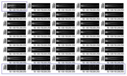
Fig. 1 All frames in the original series. Frames
circled in blue will be discarded, and correspond to the points circled
in blue in Fig. 3
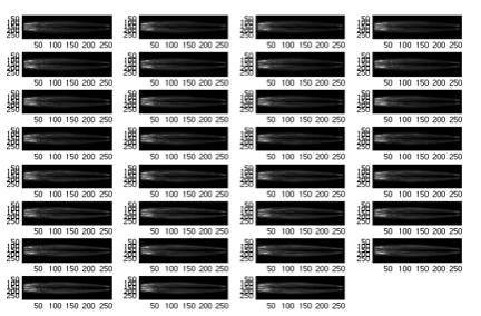
Fig. 2 Set of frames
after discarding the noisy frames. This is the set that will be used
to find the best match mask and arterial phase images.
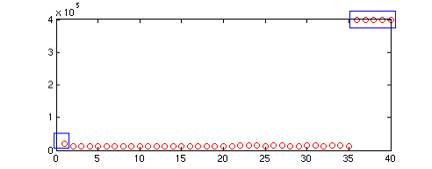
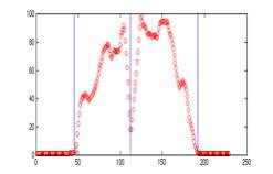
Fig. 3 This plot shows
the sum of intensities of each frame, the outliers circled in blue
correspond to the noisy frames in Fig. 1, and are discarded in Fig.
2.
2) Estimate Image Boundaries
The main purpose of this operation is to find the vertical
line (vertical defined as parallel to the legs), splitLine, where it
separates the left and the right legs. Since
the split line should reside roughly in the center of image, it is estimated
by finding the minimum column sum of intensity ( each column is a vertical
scan line) beginning from the center of the image and plus and minus
fifty pixels (columns) from the center.
The legs usually take up only a portion of the original
image, leaving parts of the left and the right side of the image empty.
Using the same information, column sum of intensity, the position of
the leg can be estimated and the images maybe reconstructed accordingly
to discard the empty portion and reduce useless calculations in the further
steps. Variable rightLine refers to the right most column that the right
leg occupies and leftLine refers the left most column that the left leg
occupies.
Because the positions of the legs are assumed to be
static, one of the frames is chosen ( the middle frame in our case) to
estimate the three lines.
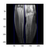
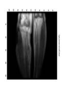
Fig 4. Each red circle in the plot is the vertical
column sum of intensity of the image on the left. The three blue lines from the left to
right in both the image and the plot refer to the leftLine, splitLine,
and the rightLine.
3) Separate the Images into rightSet and leftSet
The original images are reconstructed and separated
using the information acquired from step 2. Each
image in the rightSet contains all pixels from the righLine’th column
to the splitLine’th column from the original image and each image in
the leftSet contains all pixels from the leftLine’th column to the splitLine’th
column from the original image. Each
image is the tightest bound of the leg.
Perhaps the removal of the empty parts of the image
was responsible for the (roughly) disproportionally longer execution
time for 2 leg per image than 2 runs of single leg per image on a dual
processor 500 MHz G4 PowerPC.
4) Estimate Contrast Arrival Raj Ashish’s contrast arrival estimation algorithm is
adopted. The algorithm is
applied independently on both the rightSet and the leftSet.
5) Separate the set into maskSet and arterialPhase 6) Estimate the quality of all pairs of maskSet and
arterialPhase 7) Select the pair that yields the best quality
For each set we further divide it into the maskSet and
the arterialPhase according to the arrival of contrast estimated from
step four. The quality of
subtracted image from every pair of images in maskSet and arterilaPhase
is then computed. The best
resulting quality reveals the match of mask image and arterial phase
image that produce the best subtracted image.
The quality calculation is discussed in the next section.
Foreground Estimation and Quality Calculation
The underlying formula for estimating the quality is
adopted from (1).
The identification of foreground pixels is however different. A
new approach is proposed which requires no estimation of the minimum
and maximum width of the vessel. The
labeling scheme is discussed below.
The goal is to label each pixel p in the image to be either the foreground or the background. The
algorithm must be very efficient because while there are about 35 to
40 images in the series, the number of possible subtracted images can
be as large as a few hundred.
We first observe that for a horizontal scan line of
the image, the intensities of the pixels where arteries reside are significantly
higher than the non-artery pixels. Secondly,
we observe that the foreground, the blood vessels, should all be connected,
and most likely vertically. Therefore
for each horizontal scan line i = 2 to h, the height of
the image, we do the following :
i)
scan each pixel p( i , j ), j = 2 to w, width of the
image
ii)
if | I(p( i , j )) – I(p(
i , j - 1)) | > ∆ switch mode m. (∆ is discussed in the caveat section) where I is
the intensity of the pixel.
iii)
if m = background mode, pMap( i , j ) = 0
iv)
if m = foreground mode if pMap( i -1, j ) or pMap( i -1, j+1 ) or pMap( i -1, j - 1 ) > 0 pMap( i , j ) = 1 (a) else pMap( i -1, j ) = 0.5 (b) Using the above algorithm, a matrix, pMap, size h x w is built, where pMap( i , j
) indicates p( i , j ) being identified as foreground if pMap(
i , j ) were greater than 0. In (b) we penalize any pixel that
does not have an upper neighbor being labeled as foreground, we half
its contribution to the sum of foreground intensity; in turn, we ensure
the connectivity of the foreground, and as a2 in Fig.7 shows, it reduces
the contribution of incorrectly labeled pixels. The
starting point of vessels or any disconnected segments of vessels (real
foreground) will be halved as well, but
it’s only one out of more than two hundred foreground labels and it
still has a 0.5 contribution, therefore the impact should not be significant
to the overall calculation. The
sum of foreground intensity is therefore calculated as:
Because we have only one leg in the image, we may identify
the pixel that has the maximum intensity of each horizontal scan line,
and most of the time this point will be where the vessel resides. A map pMax is built where the pixels in the original image containing
maximum intensity of the horizontal line will have a value 1 and all
others to be zero. From
a3 of Figure 6, it can be seen that extend pMax’s labeling horizontally by one pixel to the left and right might further
enhance the result, however this was not tested in the experiment.
Using this map, pMax,
we may confirm and adjust pMap. Due to the nature of the algorithm described
above, pMap may be slightly
off position horizontally, using pMax we can adjust pMap’s position by getting
Min | pMax – pMap’ |
where pMap’ is pMap shifted a few pixels horizontally.
For confirmation, we get a final map by
finalMap = pMax + pMap’ ./ 2
If the two maps agree on the same pixel being foreground
then finalMap would keep a value one, otherwise the estimate will be
halved. Instead of doing
addition, we average the two maps because it’s not always true that the
maximum intensity of one horizontal line is where the vessel is, sometimes
noise can have the maximum intensity among the scan line. Therefore,
by average the two map, the two maps will compensate each other’s incorrect
estimations, boost pMap’s uncertain (0.5) estimations on the foregrounds and
further suppressed the background pixels that pMap was uncertain about.
This new scheme can effectively make a conservative estimation of the foreground pixels which allow us to calculate the quality of the subtracted image without the need to estimate the minimum and the maximum width of the vessel. Here we conclude our discussion on foreground estimation and quality calculation.
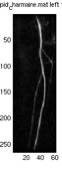
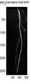
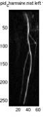
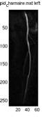
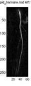
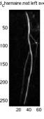
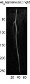
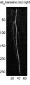
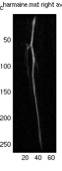
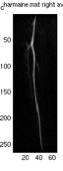
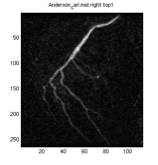
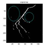
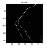
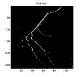
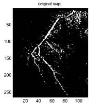
Fig. 6. a1 shows the
original image. a2 shows
the original map, pMap, produced by the algorithm without adjustment
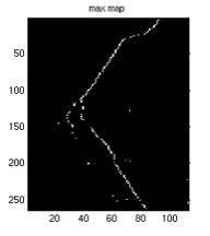
and correction by the max map, pMax. a3 shows the max map where every
point on the map is the maximum intensity of that particular horizontal
scan line (all points should have the same intensity one, the grey
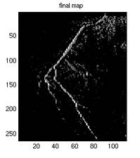
points were due to the scaling of the image). a4 is the final map used
in identifying the foreground which is the average of a2 and a3. This
example is drawn from the best subtracted image of this particular
case, where a2 has very little noise, and the noise (circled) was suppressed
after being averaged with a3, as shown in a4. It can also be seen from a3 that not all the maximum points
of a horizontal scan line is part of the vessel, therefore the averaging
may correct the point.
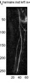
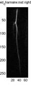
Fig. 7. Like Fig. 6, a1 shows the original image,
a2 shows the original map, a3 shows the max map, and a4 shows the final
averaged map, where this subtracted image is not in the top five choices. From a2 we can see, the neighboring system
suppresses (grey points) a lot of the noise (points that are actually
background), both the single isolated points, and the group of points
on the top right. The averaging with a3 further reduce these noise’s
contribution to ¼.
As a lesson learnt from Machine Learning, ‘bagging’
the result almost always helps. Although
the purpose of the computer algorithm is to automatically select the
best mask and arterial phase images, the ultimate goal is to produce
the best subtracted image for diagnose purpose. While it is not possible to average real physical MR images,
it is possible through digital computation.
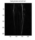
Both averaging the top three and the top five subtracted
images were attempted. It is vary obvious visually that the most averaged
images significantly reduces the noise and enhanced the vessel as seen
in a6, b6, and b7 of Figure 8. Numerically,
all three of these images yield higher quality scores. However, although numerically one was
better than the other, it is not clear visually if one is better than
the other. While the b4
and b5 scored low due to noise, they also capture some finer detail of
the vessels that are missing from the b1, b2, and b3. Including
b4, and b5 will enhance the vessels but also introduce higher noise and
lower quality score. Therefore
with averaging we again have the noise and fine detail trade off. While
a4, and a5 do not seem to have high noise, the significant high noise
in a6 is suspected be due to the off position of a4 and a5.
Further work could be done to find the best way to search
for the best averaged image. It
is not obvious how to search the best averaged images as we see from
the example. The search
space is O(n^n) where n is the number of images that can be averaged. How to determine n from the set of all
subtracted images is also another interesting topic.
*Index
(x,y) indicates the xth mask frame and the yth arterial phase image.
Fig.
8. The top portion shows
the results for the top 5 subtracted images for the left leg and averaged
image of the top3 and averaged image of the top5. The bottom portion
shows the same information for the right leg.
Fig.
9 shows the results of the top 5 subtracted images from two leg images
and averaged image of the top3.
The Use
of Single Leg Per Image
The use of
single leg per image shows that the bolus does not arrive at the same
time for the right and the left leg. For
the left leg, the bolus arrives at frame 13, and for the right leg,
the bolus arrives at frame 11. The
bolus is detected to arrive at frame 13 for the two leg images. Although
for this particular case, no arterial phase image is chosen before
the 13th frame for the top 5 subtracted images, different and better
independent matches for the two legs may potentially be missed if two
leg per image are used. We can also see that besides the top 3rd match,
the left and the right leg choose different matches of mask and arterial
phase images. While the left leg prefers the 14th frame to be the arterial
phase image, the right leg prefers the 13th.
In addition,
two leg per image suffers from motion artifacts (c4, and c5). The algorithm misidentifies the artifacts
as the foreground and scores the images incorrectly high. This problem is avoided when single leg
per image is used.
The Algorithm
In general
the algorithm successfully identifies the foreground pixel for the
evaluation of the subtracted images. The
right leg is a good example to show that the finer detail of the arterial
was sacrificed for less noise as we see (b1) has less noise and less
detail, and (b4) and (b5) have more noise but much more detail. Though
not as dramatic, the left leg also has the same effect when comparing
(a1) and (a2) where (a2) has more detail on the start shape vessels
on the top right.
Averaging
While no data from previous work is available to be
compared with, perhaps the most exciting result of the paper is the averaging
of the subtracted images, besides from the fact that the algorithm requires
no estimation of the width of the vessels. It
is not as easy to see from the images above due to scaling; however,
for the left leg, the average of the top 3 subtracted images (a6) significantly
reduces the noise on the left side of the vessels while preserves the
clarity of the vessels, and indeed it scores higher than the best non
averaged image (a1). However,
the average of the top five images (a7) significantly degrades the image. I suspect that (a4) and/or (a5) are not
perfectly inline in position with (a1), (a2), and (a3), which not only
fail to average out the noise, but introduced further noise.
For the right leg, both (b6) and (b7) significantly
reduce the noise and preserve the vessels. However,
(b7) benefited from (b4) and (b5) in that it was able to enhance the
intensity of the thinner vessels which is suppressed in (b1) (b2) and
(b3). Again the averaged
image scores higher than the best non averaged image(b1).
Averaging also helps two leg images, however only the
top 3 is averaged due to the non meaningful results of (c4) and (c5).
As noted in the foreground estimation and quality calculation
section, the algorithm relies on the detection of significant intensity
changes in a horizontal scan line. As far as the significant intensity change, the algorithm
requires an estimation of a threshold, ∆, perhaps in exchange to the
estimation of the width of the vessels. The higher the threshold is the
less noise we get, however finer detail of the correct foreground is
lost. When the threshold is low, the finer
vessels can be captured, but we also get significant noise. Empirical
results show that a threshold of 0.04 works pretty well on all cases
that had been experimented in terms of the balance between theold, or
further work will have to be done to estimate this threshold in order
to make the whole process fully automatic.
A new algorithm has been proposed to identify foreground
pixels of temporally resolved MR digital subtraction angiography for
the use of quality evaluation. The
algorithm conservatively identifies the foreground pixels without the
need to estimate the bound of foreground width. The
use of single leg per image shows that the contrast may arrive at a different
time for the two legs; furthermore it aids (at least this particular
algorithm) cases where two leg per image had difficulty producing meaningful
results due to motion artifacts. Averaging
the best subtracted results further enhances the image quality. Although no results from the previous
work are available for comparison, and no double blind experiment is
conducted, the results seem to be competitive.
As eluded from previous sections, it is useful to develop
an algorithm that can search for the best threshold. While averaging the best subtracted images enhances images
even further, an efficient algorithm is needed to search for the best
averaged image. As mentioned,
the max map may be improved by expanding its labeling horizontally, but
the effect is yet to be determined. Last
but not least, the POCS algorithm may be applied on the images that are
discarded in step one, perhaps these images might be even better choices
of the mask and/or the arterial phase images.
1. Kim, J. et al. Automatic Selection of Mask and Arterial
Phase Images for Temporally Resolved MR Digital Subtraction Angiography. Magnetic Resonance in Medicine 48:1004-1010(2002)
|
|||||||||||||||||||||||||||||||||||||||||||||||||||||||||||||||||||||||||||||||||||||||||||||||||||||||||||||||||||||||||||||||||||

 a1
a1
 a2
a2
 a3
a3
 a4
a4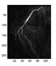 a1
a1
 a3
a3
 a4
a4