Prev: L23, Next: L25, Zoom: Link
Wisc NetID for In-class Quiz: @wisc.edu
4-digit Passcode: (anything is okay, use the same one for all lectures or use based on your id)
Save submission to file? File name: (leave it blank to not save anything) 24 id,answer_id;token,answer_check;download,answer_download
Slide:
# Deep Q Learning
📗 In practice, Q function stored as a table is too large if the number of states is large or infinite (the action space is usually finite): Link, Link, Wikipedia.
📗 If there are \(m\) binary features that represent the state, then the Q table contains \(2^{m} \left| A \right|\), which can be intractable.
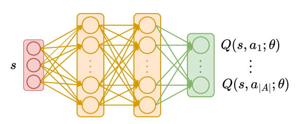
📗 In this case, a neural network can be used to store the Q function, and if there is a single layer with \(m\) units, then only \(m^{2} + m \left| A \right|\) weights are needed.
➩ The input of the network \(\hat{Q}\) is the features of the state \(s\), and the outputs of the network are Q values associated with the actions \(a\) or \(Q\left(s, a\right)\) (the output layer does not need to be softmax since the Q values for different actions do not need to sum up to \(1\)).
➩ After every iteration, the network can be updated based on an item \(\left(s_{t}, \left(1 - \alpha\right) \hat{Q}\left(s_{t}, a_{t}\right) + \alpha \left(r_{t} + \beta \displaystyle\max_{a} \hat{Q}\left(s_{t+1}, a\right)\right)\right)\).
# Deep Q Network
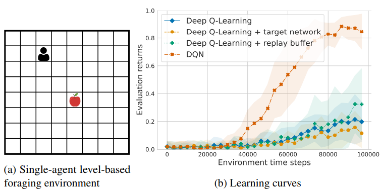
📗 Deep Q Learning algorithm is unstable since the training label uses the network itself. The following improvements can be made to make the algorithm more stable, called DQN (Deep Q Network).
➩ Target network: two networks can be used, the Q network \(\hat{Q}\) and the target network \(Q'\), and the new item for training \(\hat{Q}\) can be changed to \(\left(s_{t}, \left(1 - \alpha\right) Q'\left(s_{t}, a_{t}\right) + \alpha \left(r_{t} + \beta \displaystyle\max_{a} Q'\left(s_{t+1}, a\right)\right)\right)\).
➩ Experience replay: some training data can be saved and a mini-batch (sampled from the training set) can be used to update \(\hat{Q}\) instead of a single item.
Example
# Policy Gradient
📗 Deep Q Network estimates the Q function as a neural network, and the policy can be computed as \(\pi\left(s\right) = \mathop{\mathrm{argmax}}_{a} \hat{Q}\left(s, a\right)\), which is always deterministic.
➩ In single-agent reinforcement learning, there is always a deterministic optimal policy, so DQN can be used to solve for an optimal policy.
➩ In multi-agent reinforcement learning, the optimal equilibrium policy can be all stochastic (mixed strategy equilibrium): Wikipedia.
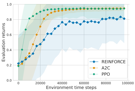
📗 The policy can also be represented by a neural network called the policy network \(\hat{\pi}\) and it can be trained with or without using a value network \(\hat{V}\).
➩ Without a value network: REINFORCE (REward Increment = Non-negative Factor x Offset x Characteristic Eligibility).
➩ With a value network: A2C (Advantage Actor Critic) and PPO (Proximal Policy Optimization).
📗 To train the policy network \(\hat{\pi}\), the input is the features of the state \(s\) and the output units (softmax output layer) are the probability of using each action \(a\) or \(\mathbb{P}\left\{\pi\left(s\right) = a\right\}\). The cost function the network minimizes can be value function (REINFORCE) or the advantage function (difference between value and Q, A2C and PPO).
📗 The value network is trained in a way similar to DQN.
Example
Math Note
📗 Policy gradient theorem: \(\nabla_{w} V\left(w\right) = \mathbb{E}\left[Q^{\hat{\pi}}\left(s, a\right) \nabla_{w} \log \hat{\pi}\left(a | s; w\right)\right]\)
➩ Given this gradient formula, the loss for the policy network in REINFORCE can be written as \(\left(\displaystyle\sum_{t'=t+1}^{T} \beta^{t'-t-1} r_{t'}\right) \log \pi\left(a_{t} | s_{t} ; w\right)\), where \(\displaystyle\sum_{t'=t+1}^{T} \beta^{t'-t-1} r_{t'}\) is an estimate of \(Q^{\hat{\pi}}\left(s_{t}, a_{t}\right)\).
➩ The loss for the policy network in A2C is \(-\left(r_{t} + \beta \hat{V}\left(s_{t+1}\right) - \hat{V}\left(s_{t}\right)\right) \log \pi\left(a_{t} | s_{t} ; w\right)\), where \(r_{t} + \beta \hat{V}\left(s_{t+1}\right) - \hat{V}\left(s_{t}\right)\) is an estimate of the advantage function \(Q^{\hat{\pi}}\left(s_{t}, a_{t}\right) - V^{\hat{\pi}}\left(s_{t}\right)\).
# Questions?
📗 If you have questions, please (i) Ask during or after the lecture or the break, (ii) Piazza: Link, (iii) Office hours and discussion sessions. Please do NOT use Canvas mail and use email only to the course instructor (not TAs) for grading issues.
Additional In-class Discussion
📗 Sometimes a question not in the notes will be asked during the lecture, you can submit your answer here:
[Notes] (not visible to other students):
[L24Q1]
Submit your answer to see other students answers (click the submit button to refresh):
Additional In-class Quiz
📗 Sometimes a question not in the notes will be asked during the lecture, you can submit your answer here:
A. B.
C.
D.
E.
[Notes] (not visible to other students):
[L24Q2]
Submit your answer to see other students answers (click the submit button to refresh):
test q https://script.google.com/macros/s/AKfycbyiidUAdiLc3YrKgOAM6T95ATulwDQxQilWVv1bK1L5sKRl8ozXfVs4PjCC2VtMWcIBpg/exec
# In-class Quiz Instructions
📗 To get full points on the in-class quizzes for a lecture:
➩ Submit relevant answers to the questions discussed during the lecture: incorrect answers are okay.
➩ Some questions require [notes] to earn the point.
➩ Some questions require special ID (given during the lecture) to earn the point.
➩ Do not submit answers to questions that are not discussed during the lectures. Each such submission will result in a deduction of one point.
➩ The grade on Canvas Assignment W24 is computed as number of points divided by the number of questions asked (and multiplied by 4, out of 4) and updated on Canvas every weekend.
📗 Notes and code adapted from the course taught by Professors Jerry Zhu, Blerina Gkotse, Yudong Chen, Yingyu Liang, Charles Dyer. Some content are generated using Copilot .
Prev: L23, Next: L25
Last Updated: October 15, 2026 at 2:54 AM