Prev: L3, Next: L5, Zoom: Link
Wisc NetID for In-class Quiz: @wisc.edu
4-digit Passcode: (anything is okay, use the same one for all lectures or use based on your id)
Save submission to file? File name: (leave it blank to not save anything) 4 id,answer_id;token,answer_check;download,answer_download
Slide:
# Gradient Descent
📗 Gradient descent will be used, and the gradient will be computed using chain rule. The algorithm is called backpropogation: Wikipedia.
📗 For a neural network with one input layer, one hidden layer, and one output layer:
➩ \(\dfrac{\partial C_{i}}{\partial w_{j}^{\left(2\right)}} = \dfrac{\partial C_{i}}{\partial a_{i}^{\left(2\right)}} \dfrac{\partial a_{i}^{\left(2\right)}}{\partial w_{j}^{\left(2\right)}}\), for \(j = 1, 2, ..., m^{\left(1\right)}\).
➩ \(\dfrac{\partial C_{i}}{\partial b^{\left(2\right)}} = \dfrac{\partial C_{i}}{\partial a_{i}^{\left(2\right)}} \dfrac{\partial a_{i}^{\left(2\right)}}{\partial b^{\left(2\right)}}\).
➩ \(\dfrac{\partial C_{i}}{\partial w_{j' j}^{\left(1\right)}} = \dfrac{\partial C_{i}}{\partial a_{i}^{\left(2\right)}} \dfrac{\partial a_{i}^{\left(2\right)}}{\partial a_{ij}^{\left(1\right)}} \dfrac{\partial a_{ij}^{\left(1\right)}}{\partial w_{j' j}^{\left(1\right)}}\), for \(j' = 1, 2, ..., m, j = 1, 2, ..., m^{\left(1\right)}\).
➩ \(\dfrac{\partial C_{i}}{\partial b_{j}^{\left(1\right)}} = \dfrac{\partial C_{i}}{\partial a_{i}^{\left(2\right)}} \dfrac{\partial a_{i}^{\left(2\right)}}{\partial a_{ij}^{\left(1\right)}} \dfrac{\partial a_{ij}^{\left(1\right)}}{\partial b_{j}^{\left(1\right)}}\), for \(j = 1, 2, ..., m^{\left(1\right)}\).
📗 More generally, the derivatives can be computed recursively.
➩ \(\dfrac{\partial C_{i}}{\partial b_{j}^{\left(l\right)}} = \left(\dfrac{\partial C_{i}}{\partial b_{1}^{\left(l + 1\right)}} w_{j 1}^{\left(l+1\right)} + \dfrac{\partial C_{i}}{\partial b_{2}^{\left(l + 1\right)}} w_{j 2}^{\left(l+1\right)} + ... + \dfrac{\partial C_{i}}{\partial b_{m^{\left(l + 1\right)}}^{\left(l + 1\right)}} w_{j m^{\left(l + 1\right)}}^{\left(l+1\right)}\right) g'\left(a^{\left(l\right)}_{i j}\right)\), where \(\dfrac{\partial C_{i}}{\partial b^{\left(L\right)}} = \dfrac{\partial C_{i}}{\partial a_{i}^{\left(L\right)}} g'\left(a_{i}^{\left(L\right)}\right)\).
➩ \(\dfrac{\partial C_{i}}{\partial w_{j' j}^{\left(l\right)}} = \dfrac{\partial C_{i}}{\partial b_{j}^{\left(l\right)}} a_{i j'}^{\left(l - 1\right)}\).
📗 Gradient descent formula is the same: \(w = w - \alpha \left(\nabla_{w} C_{1} + \nabla_{w} C_{2} + ... + \nabla_{w} C_{n}\right)\) and \(b = b - \alpha \left(\nabla_{b} C_{1} + \nabla_{b} C_{2} + ... + \nabla_{b} C_{n}\right)\) for all the weights and biases.
Example
📗 PyTorch code example: Link.
📗 For two layer neural network with sigmoid activations (used in logistic regression) and square loss,
➩ The
\(a^{\left(1\right)}_{ij} = \dfrac{1}{1 + \exp\left(- \left(\left(\displaystyle\sum_{j'=1}^{m} x_{ij'} w^{\left(1\right)}_{j'j}\right) + b^{\left(1\right)}_{j}\right)\right)}\) for j = 1, ..., h, forward() step in PyTorch: \(a^{\left(2\right)}_{i} = \dfrac{1}{1 + \exp\left(- \left(\left(\displaystyle\sum_{j=1}^{h} a^{\left(1\right)}_{ij} w^{\left(2\right)}_{j}\right) + b^{\left(2\right)}\right)\right)}\),
➩ The
\(\dfrac{\partial C_{i}}{\partial w^{\left(1\right)}_{j'j}} = \left(a^{\left(2\right)}_{i} - y_{i}\right) a^{\left(2\right)}_{i} \left(1 - a^{\left(2\right)}_{i}\right) w_{j}^{\left(2\right)} a_{ij}^{\left(1\right)} \left(1 - a_{ij}^{\left(1\right)}\right) x_{ij'}\) for j' = 1, ..., m, j = 1, ..., h, backward() step in PyTorch: \(\dfrac{\partial C_{i}}{\partial b^{\left(1\right)}_{j}} = \left(a^{\left(2\right)}_{i} - y_{i}\right) a^{\left(2\right)}_{i} \left(1 - a^{\left(2\right)}_{i}\right) w_{j}^{\left(2\right)} a_{ij}^{\left(1\right)} \left(1 - a_{ij}^{\left(1\right)}\right)\) for j = 1, ..., h,
\(\dfrac{\partial C_{i}}{\partial w^{\left(2\right)}_{j}} = \left(a^{\left(2\right)}_{i} - y_{i}\right) a^{\left(2\right)}_{i} \left(1 - a^{\left(2\right)}_{i}\right) a_{ij}^{\left(1\right)}\) for j = 1, ..., h,
\(\dfrac{\partial C_{i}}{\partial b^{\left(2\right)}} = \left(a^{\left(2\right)}_{i} - y_{i}\right) a^{\left(2\right)}_{i} \left(1 - a^{\left(2\right)}_{i}\right)\),
\(w^{\left(1\right)}_{j' j} \leftarrow w^{\left(1\right)}_{j' j} - \alpha \dfrac{\partial C_{i}}{\partial w^{\left(1\right)}_{j' j}}\) for j' = 1, ..., m, j = 1, ..., h,
\(b^{\left(1\right)}_{j} \leftarrow b^{\left(1\right)}_{j} - \alpha \dfrac{\partial C_{i}}{\partial b^{\left(1\right)}_{j}}\) for j = 1, ..., h,
\(w^{\left(2\right)}_{j} \leftarrow w^{\left(2\right)}_{j} - \alpha \dfrac{\partial C_{i}}{\partial w^{\left(2\right)}_{j}}\) for j = 1, ..., h,
\(b^{\left(2\right)} \leftarrow b^{\left(2\right)} - \alpha \dfrac{\partial C_{i}}{\partial b^{\left(2\right)}}\).
In-class Quiz
📗 Highlight the weights used in computing \(\dfrac{\partial C}{\partial w^{\left(1\right)}_{11}}\) in the backpropogation step.
📗 [1 points] The following is a diagram of a neural network: highlight an edge (mouse or touch drag from one node to another node) to see the name of the weight (highlight the same edge to hide the name). Highlight color: .
Name of input units: 4
Name of hidden layer 1 units: 3
Name of hidden layer 2 units: 2
Name of hidden layer 3 units: 0
Name of output units: 1
1 slider
# Stochastic Gradient Descent
📗 The gradient descent algorithm updates the weight using the gradient which is the sum over all items, for logistic regression: \(w = w - \alpha \left(\left(a_{1} - y_{1}\right) x_{1} + \left(a_{2} - y_{2}\right) x_{2} + ... + \left(a_{n} - y_{n}\right) x_{n}\right)\).
📗 A variant of the gradient descent algorithm that updates the weight for one item at a time is called stochastic gradient descent. This is because the expected value of \(\dfrac{\partial C_{i}}{\partial w}\) for a random \(i\) is equal to \(\dfrac{\partial C}{\partial w}\): Wikipedia.
➩ Gradient descent (batch): \(w = w - \alpha \dfrac{\partial C}{\partial w}\) or \(w = w - \alpha \left(\dfrac{\partial C_{1}}{\partial w} + \dfrac{\partial C_{2}}{\partial w} + ... + \dfrac{\partial C_{n}}{\partial w}\right)\).
➩ Stochastic gradient descent: for a random \(i \in \left\{1, 2, ..., n\right\}\), \(w = w - \alpha \dfrac{\partial C_{i}}{\partial w}\).
📗 Instead of randomly pick one item at a time, the training set is usually shuffled, and the shuffled items will be used to update the weights and biases in order. Looping through all items once is called an epoch.
➩ Stochastic gradient descent can also help moving out of a local minimum of the cost function: Link.
Example
📗 [1 points] Suppose the minimum occurs at the center of the plot: the following are paths based on (batch) gradient descent [red] vs stochastic gradient descent [blue]. Move the green point to change the starting point.
Math Note
📗 Note: the Perceptron algorithm updates the weight for one item at a time: \(w = w - \alpha \left(a_{i} - y_{i}\right) x_{i}\), but it is not gradient descent or stochastic gradient descent.
# Softmax Layer
📗 For both logistic regression and neural network, the output layer can have \(K\) units, \(a_{i k}^{\left(L\right)}\), for \(k = 1, 2, ..., K\), for K-class classification problems: Link,
📗 The labels should be converted to one-hot encoding, \(y_{i k} = 1\) when the true label is \(k\) and \(y_{i k} = 0\) otherwise.
➩ If there are \(K = 3\) classes, then all items with true label \(1\) should be converted to \(y_{i} = \begin{bmatrix} 1 \\ 0 \\ 0 \end{bmatrix}\), and true label \(2\) to \(y_{i} = \begin{bmatrix} 0 \\ 1 \\ 0 \end{bmatrix}\), and true label \(3\) to \(y_{i} = \begin{bmatrix} 0 \\ 0 \\ 1 \end{bmatrix}\).
📗 The last layer should normalize the sum of all \(K\) units to \(1\). A popular choice is the softmax operation: \(a_{i k}^{\left(L\right)} = \dfrac{e^{z_{i k}}}{e^{z_{i 1}} + e^{z_{i 2}} + ... + e^{z_{i K}}}\), where \(z_{i k} = w_{1 k} a_{i 1}^{\left(L - 1\right)} + w_{2 k} a_{i 2}^{\left(L - 1\right)} + ... w_{m^{\left(L - 1\right)} k} a_{i m^{\left(L - 1\right)}}^{\left(L - 1\right)} + b_{k}\) for \(k = 1, 2, ..., K\): Wikipedia.
Example
📗 [1 points] The following is a diagram of a neural network: highlight an edge (mouse or touch drag from one node to another node) to see the name of the weight (highlight the same edge to hide the name). Highlight color: .
Name of input units: 4
Name of hidden layer 1 units: 3
Name of hidden layer 2 units: 2
Name of hidden layer 3 units: 0
Name of output units: 1
1 slider
Math Note
📗 If cross entropy loss is used, \(C_{i} = -y_{i 1} \log\left(a_{i 1}\right) - y_{i 2} \log\left(a_{i 2}\right) + ... - y_{i K} \log\left(a_{i K}\right)\), then the derivative can be simplified to \(\dfrac{\partial C_{i}}{\partial z_{i k}} = a^{\left(L\right)}_{i k} - y_{i k}\) or \(\nabla_{z_{i}} C_{i} = a^{\left(L\right)}_{i} - y_{i}\).
➩ Some calculus:
\(C_{i} = - \displaystyle\sum_{k=1}^{K} y_{i k} \log \dfrac{e^{z_{i k}}}{\displaystyle\sum_{k' = 1}^{K} e^{z_{i k'}}}\) \(= \displaystyle\sum_{k=1}^{K} y_{i k} \log \left(\displaystyle\sum_{k=1}^{K} e^{z_{i k}}\right) - \displaystyle\sum_{k=1}^{K} y_{i k} z_{i k}\)
\(= \log \left(\displaystyle\sum_{k=1}^{K} e^{z_{i k}}\right) - \displaystyle\sum_{k=1}^{K} y_{i k} z_{i k}\) since \(y_{i k}\) sum up to \(1\) for a fixed item \(i\).
\(\dfrac{\partial C_{i}}{\partial z_{i k}} = \dfrac{e^{z_{i k}}}{\displaystyle\sum_{k' = 1}^{K} e^{z_{i k'}}} - y_{i k} = a^{\left(L\right)}_{i k} - y_{i k}\)
\(\nabla_{z_{i}} C_{i} = a^{\left(L\right)}_{i} - y_{i}\).
# Function Approximator
📗 Neural networks can be used in different areas of machine learning.
➩ In supervised learning, a neural network approximates \(\mathbb{P}\left\{y | x\right\}\) as a function of \(x\).
➩ In unsupervised learning, a neural network can be used to perform non-linear dimensionality reduction. Training a neural network with output \(y_{i} = x_{i}\) and fewer hidden units than input units will find a lower dimensional representation (the values of the hidden units) of the inputs. This is called an auto-encoder: Wikipedia.
➩ In reinforcement learning, there can be multiple neural networks to store and approximate the value function and the optimal policy (choice of actions): Wikipedia.
# Generalization Error
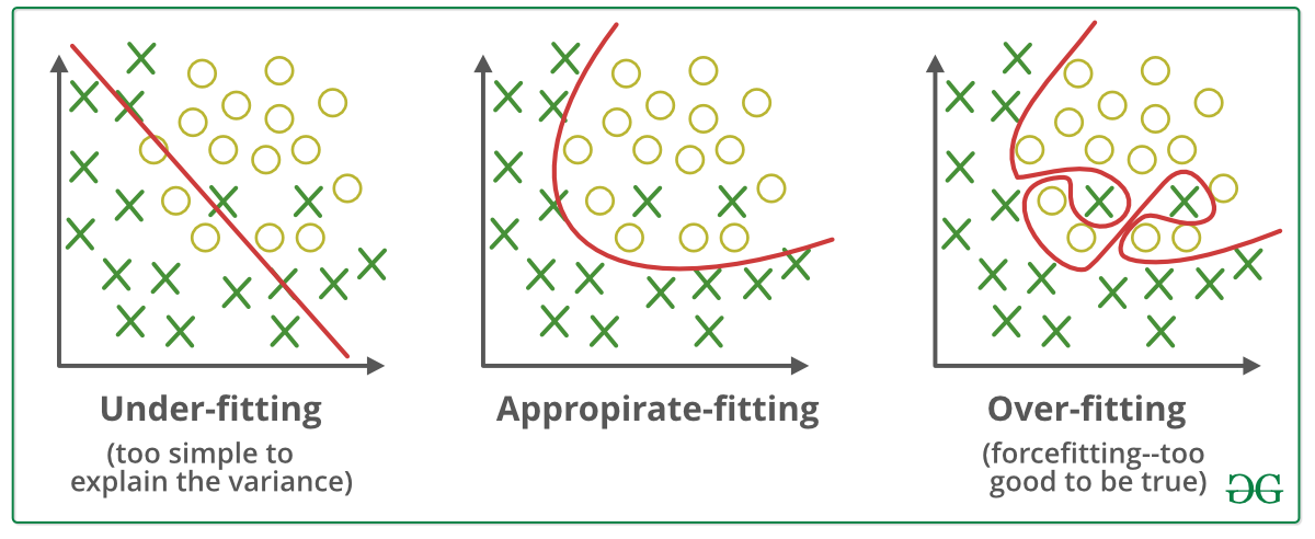
📗 With a large number of hidden layers and units, a neural network can overfit a training set perfectly. This does not imply the performance on new items will be good: Wikipedia.
➩ More data can be created for training using generative models or unsupervised learning techniques.
➩ A validation set can be used (similar to pruning for decision trees) to train the network until the loss (or accuracy) on the validation set begins to increase.
➩ Dropout can be used: randomly omitting units (random pruning of weights) during training so the rest of the units will have a better performance: Wikipedia.
Example
# Regularization
📗 A simpler model (with fewer weights, or many weights set to 0) is usually more generalizable and would not overfit the training set as much. A way to achieve that is to include an additional cost for non-zero weights during training. This is called regularization: Wikipedia.
➩ \(L_{1}\) regularization adds \(L_{1}\) norm of the weights and biases to the loss, or \(C = C_{1} + C_{2} + ... + C_{n} + \lambda \left\|\begin{bmatrix} w \\ b \end{bmatrix}\right\|_{1}\), for example, if there are no hidden layers, \(\left\|\begin{bmatrix} w \\ b \end{bmatrix}\right\|_{1} = \left| w_{1} \right| + \left| w_{2} \right| + ... + \left| w_{m} \right| + \left| b \right|\). Linear regression with \(L_{1}\) regularization is also called LASSO (Least Absolute Shrinkage and Selector Operator): Wikipedia.
➩ \(L_{2}\) regularization adds \(L_{2}\) norm of the weights and biases to the loss, or \(C = C_{1} + C_{2} + ... + C_{n} + \lambda \left\|\begin{bmatrix} w \\ b \end{bmatrix}\right\|^{2}_{2}\), for example, if there are no hidden layers, \(\left\|\begin{bmatrix} w \\ b \end{bmatrix}\right\|^{2}_{2} = \left(w_{1}\right)^{2} + \left(w_{2}\right)^{2} + ... + \left(w_{m}\right)^{2} + \left(b\right)^{2}\). Linear regression with \(L_{2}\) regularization is also called ridge regression: Wikipedia.
📗 \(\lambda\) is chosen as the trade-off between the loss from incorrect prediction and the loss from non-zero weights.
➩ \(L_{1}\) regularization often leads to more weights that are exactly \(0\), which is useful for feature selection.
➩ \(L_{2}\) regularization is easier for gradient descent since it is differentiable.
➩ Try \(L_{1}\) vs \(L_{2}\) regularization here: Link.
In-class Discussion
📗 [1 points] Fix some \(d\), find the point where \(\left\|\begin{bmatrix} w_{1} \\ w_{2} \end{bmatrix}\right\| \leq d\) and minimize the cost \(c\). Use regularization.
➩ Aside: compare the above procedure with: fix some cost \(c\), find the point with the minimum distance to the origin \(d\). This is related to this duality of optimization.
Bound \(d\): 0.5
Cost \(C\): 0
1 slider
[L4Q2]
# Questions?
📗 If you have questions, please (i) Ask during or after the lecture or the break, (ii) Piazza: Link, (iii) Office hours and discussion sessions. Please do NOT use Canvas mail and use email only to the course instructor (not TAs) for grading issues.
Additional In-class Discussion
📗 Sometimes a question not in the notes will be asked during the lecture, you can submit your answer here:
[Notes] (not visible to other students):
[L4Q3]
Submit your answer to see other students answers (click the submit button to refresh):
Additional In-class Quiz
📗 Sometimes a question not in the notes will be asked during the lecture, you can submit your answer here:
A. B.
C.
D.
E.
[Notes] (not visible to other students):
[L4Q4]
Submit your answer to see other students answers (click the submit button to refresh):
test nnd,sgd,sfm,rd q https://script.google.com/macros/s/AKfycbyiidUAdiLc3YrKgOAM6T95ATulwDQxQilWVv1bK1L5sKRl8ozXfVs4PjCC2VtMWcIBpg/exec
# In-class Quiz Instructions
📗 To get full points on the in-class quizzes for a lecture:
➩ Submit relevant answers to the questions discussed during the lecture: incorrect answers are okay.
➩ Some questions require [notes] to earn the point.
➩ Some questions require special ID (given during the lecture) to earn the point.
➩ Do not submit answers to questions that are not discussed during the lectures. Each such submission will result in a deduction of one point.
➩ The grade on Canvas Assignment W4 is computed as number of points divided by the number of questions asked (and multiplied by 4, out of 4) and updated on Canvas every weekend.
📗 Notes and code adapted from the course taught by Professors Jerry Zhu, Blerina Gkotse, Yudong Chen, Yingyu Liang, Charles Dyer. Some content are generated using Copilot .
Prev: L3, Next: L5
Last Updated: September 25, 2026 at 2:23 AM