Prev: L3, Next: L5
Zoom: Link, Piazza: Link, Google Form: Link.
Wisc ID for in-class quiz: (if your wisc email is "test@wisc.edu", please enter "test")
Token: (will be given during the lectures)
4
id,answer_id;token,answer_check
Slide:
# Gradient Descent
📗 Gradient descent will be used, and the gradient will be computed using chain rule. The algorithm is called backpropogation: Wikipedia.
📗 For a neural network with one input layer, one hidden layer, and one output layer:
➩ \(\dfrac{\partial C_{i}}{\partial w_{j}^{\left(2\right)}} = \dfrac{\partial C_{i}}{\partial a_{i}^{\left(2\right)}} \dfrac{\partial a_{i}^{\left(2\right)}}{\partial w_{j}^{\left(2\right)}}\), for \(j = 1, 2, ..., m^{\left(1\right)}\).
➩ \(\dfrac{\partial C_{i}}{\partial b^{\left(2\right)}} = \dfrac{\partial C_{i}}{\partial a_{i}^{\left(2\right)}} \dfrac{\partial a_{i}^{\left(2\right)}}{\partial b^{\left(2\right)}}\).
➩ \(\dfrac{\partial C_{i}}{\partial w_{j' j}^{\left(1\right)}} = \dfrac{\partial C_{i}}{\partial a_{i}^{\left(2\right)}} \dfrac{\partial a_{i}^{\left(2\right)}}{\partial a_{ij}^{\left(1\right)}} \dfrac{\partial a_{ij}^{\left(1\right)}}{\partial w_{j' j}^{\left(1\right)}}\), for \(j' = 1, 2, ..., m, j = 1, 2, ..., m^{\left(1\right)}\).
➩ \(\dfrac{\partial C_{i}}{\partial b_{j}^{\left(1\right)}} = \dfrac{\partial C_{i}}{\partial a_{i}^{\left(2\right)}} \dfrac{\partial a_{i}^{\left(2\right)}}{\partial a_{ij}^{\left(1\right)}} \dfrac{\partial a_{ij}^{\left(1\right)}}{\partial b_{j}^{\left(1\right)}}\), for \(j = 1, 2, ..., m^{\left(1\right)}\).
📗 More generally, the derivatives can be computed recursively.
➩ \(\dfrac{\partial C_{i}}{\partial b_{j}^{\left(l\right)}} = \left(\dfrac{\partial C_{i}}{\partial b_{1}^{\left(l + 1\right)}} w_{j 1}^{\left(l+1\right)} + \dfrac{\partial C_{i}}{\partial b_{2}^{\left(l + 1\right)}} w_{j 2}^{\left(l+1\right)} + ... + \dfrac{\partial C_{i}}{\partial b_{m^{\left(l + 1\right)}}^{\left(l + 1\right)}} w_{j m^{\left(l + 1\right)}}^{\left(l+1\right)}\right) g'\left(a^{\left(l\right)}_{i j}\right)\), where \(\dfrac{\partial C_{i}}{\partial b^{\left(L\right)}} = \dfrac{\partial C_{i}}{\partial a_{i}^{\left(L\right)}} g'\left(a_{i}^{\left(L\right)}\right)\).
➩ \(\dfrac{\partial C_{i}}{\partial w_{j' j}^{\left(l\right)}} = \dfrac{\partial C_{i}}{\partial b_{j}^{\left(l\right)}} a_{i j'}^{\left(l - 1\right)}\).
📗 Gradient descent formula is the same: \(w = w - \alpha \left(\nabla_{w} C_{1} + \nabla_{w} C_{2} + ... + \nabla_{w} C_{n}\right)\) and \(b = b - \alpha \left(\nabla_{b} C_{1} + \nabla_{b} C_{2} + ... + \nabla_{b} C_{n}\right)\) for all the weights and biases.
Example
📗 PyTorch code example: Link.
📗 For two layer neural network with sigmoid activations (used in logistic regression) and square loss,
➩ The
\(a^{\left(1\right)}_{ij} = \dfrac{1}{1 + \exp\left(- \left(\left(\displaystyle\sum_{j'=1}^{m} x_{ij'} w^{\left(1\right)}_{j'j}\right) + b^{\left(1\right)}_{j}\right)\right)}\) for j = 1, ..., h, forward() step in PyTorch: \(a^{\left(2\right)}_{i} = \dfrac{1}{1 + \exp\left(- \left(\left(\displaystyle\sum_{j=1}^{h} a^{\left(1\right)}_{ij} w^{\left(2\right)}_{j}\right) + b^{\left(2\right)}\right)\right)}\),
➩ The
\(\dfrac{\partial C_{i}}{\partial w^{\left(1\right)}_{j'j}} = \left(a^{\left(2\right)}_{i} - y_{i}\right) a^{\left(2\right)}_{i} \left(1 - a^{\left(2\right)}_{i}\right) w_{j}^{\left(2\right)} a_{ij}^{\left(1\right)} \left(1 - a_{ij}^{\left(1\right)}\right) x_{ij'}\) for j' = 1, ..., m, j = 1, ..., h, backward() step in PyTorch: \(\dfrac{\partial C_{i}}{\partial b^{\left(1\right)}_{j}} = \left(a^{\left(2\right)}_{i} - y_{i}\right) a^{\left(2\right)}_{i} \left(1 - a^{\left(2\right)}_{i}\right) w_{j}^{\left(2\right)} a_{ij}^{\left(1\right)} \left(1 - a_{ij}^{\left(1\right)}\right)\) for j = 1, ..., h,
\(\dfrac{\partial C_{i}}{\partial w^{\left(2\right)}_{j}} = \left(a^{\left(2\right)}_{i} - y_{i}\right) a^{\left(2\right)}_{i} \left(1 - a^{\left(2\right)}_{i}\right) a_{ij}^{\left(1\right)}\) for j = 1, ..., h,
\(\dfrac{\partial C_{i}}{\partial b^{\left(2\right)}} = \left(a^{\left(2\right)}_{i} - y_{i}\right) a^{\left(2\right)}_{i} \left(1 - a^{\left(2\right)}_{i}\right)\),
\(w^{\left(1\right)}_{j' j} \leftarrow w^{\left(1\right)}_{j' j} - \alpha \dfrac{\partial C_{i}}{\partial w^{\left(1\right)}_{j' j}}\) for j' = 1, ..., m, j = 1, ..., h,
\(b^{\left(1\right)}_{j} \leftarrow b^{\left(1\right)}_{j} - \alpha \dfrac{\partial C_{i}}{\partial b^{\left(1\right)}_{j}}\) for j = 1, ..., h,
\(w^{\left(2\right)}_{j} \leftarrow w^{\left(2\right)}_{j} - \alpha \dfrac{\partial C_{i}}{\partial w^{\left(2\right)}_{j}}\) for j = 1, ..., h,
\(b^{\left(2\right)} \leftarrow b^{\left(2\right)} - \alpha \dfrac{\partial C_{i}}{\partial b^{\left(2\right)}}\).
In-class Quiz
📗 Highlight the weights used in computing \(\dfrac{\partial C}{\partial w^{\left(1\right)}_{11}}\) in the backpropogation step.
📗 [1 points] The following is a diagram of a neural network: highlight an edge (mouse or touch drag from one node to another node) to see the name of the weight (highlight the same edge to hide the name). Highlight color: .
Name of input units: 4
Name of hidden layer 1 units: 3
Name of hidden layer 2 units: 2
Name of hidden layer 3 units: 0
Name of output units: 1
1 slider
# Stochastic Gradient Descent
📗 The gradient descent algorithm updates the weight using the gradient which is the sum over all items, for logistic regression: \(w = w - \alpha \left(\left(a_{1} - y_{1}\right) x_{1} + \left(a_{2} - y_{2}\right) x_{2} + ... + \left(a_{n} - y_{n}\right) x_{n}\right)\).
📗 A variant of the gradient descent algorithm that updates the weight for one item at a time is called stochastic gradient descent. This is because the expected value of \(\dfrac{\partial C_{i}}{\partial w}\) for a random \(i\) is equal to \(\dfrac{\partial C}{\partial w}\): Wikipedia.
➩ Gradient descent (batch): \(w = w - \alpha \dfrac{\partial C}{\partial w}\) or \(w = w - \alpha \left(\dfrac{\partial C_{1}}{\partial w} + \dfrac{\partial C_{2}}{\partial w} + ... + \dfrac{\partial C_{n}}{\partial w}\right)\).
➩ Stochastic gradient descent: for a random \(i \in \left\{1, 2, ..., n\right\}\), \(w = w - \alpha \dfrac{\partial C_{i}}{\partial w}\).
📗 Instead of randomly pick one item at a time, the training set is usually shuffled, and the shuffled items will be used to update the weights and biases in order. Looping through all items once is called an epoch.
➩ Stochastic gradient descent can also help moving out of a local minimum of the cost function: Link.
Example
📗 [1 points] Suppose the minimum occurs at the center of the plot: the following are paths based on (batch) gradient descent [red] vs stochastic gradient descent [blue]. Move the green point to change the starting point.
Math Note
📗 Note: the Perceptron algorithm updates the weight for one item at a time: \(w = w - \alpha \left(a_{i} - y_{i}\right) x_{i}\), but it is not gradient descent or stochastic gradient descent.
# Softmax Layer
📗 For both logistic regression and neural network, the output layer can have \(K\) units, \(a_{i k}^{\left(L\right)}\), for \(k = 1, 2, ..., K\), for K-class classification problems: Link,
📗 The labels should be converted to one-hot encoding, \(y_{i k} = 1\) when the true label is \(k\) and \(y_{i k} = 0\) otherwise.
➩ If there are \(K = 3\) classes, then all items with true label \(1\) should be converted to \(y_{i} = \begin{bmatrix} 1 \\ 0 \\ 0 \end{bmatrix}\), and true label \(2\) to \(y_{i} = \begin{bmatrix} 0 \\ 1 \\ 0 \end{bmatrix}\), and true label \(3\) to \(y_{i} = \begin{bmatrix} 0 \\ 0 \\ 1 \end{bmatrix}\).
📗 The last layer should normalize the sum of all \(K\) units to \(1\). A popular choice is the softmax operation: \(a_{i k}^{\left(L\right)} = \dfrac{e^{z_{i k}}}{e^{z_{i 1}} + e^{z_{i 2}} + ... + e^{z_{i K}}}\), where \(z_{i k} = w_{1 k} a_{i 1}^{\left(L - 1\right)} + w_{2 k} a_{i 2}^{\left(L - 1\right)} + ... w_{m^{\left(L - 1\right)} k} a_{i m^{\left(L - 1\right)}}^{\left(L - 1\right)} + b_{k}\) for \(k = 1, 2, ..., K\): Wikipedia.
Example
📗 [1 points] The following is a diagram of a neural network: highlight an edge (mouse or touch drag from one node to another node) to see the name of the weight (highlight the same edge to hide the name). Highlight color: .
Name of input units: 4
Name of hidden layer 1 units: 3
Name of hidden layer 2 units: 2
Name of hidden layer 3 units: 0
Name of output units: 1
1 slider
Math Note
📗 If cross entropy loss is used, \(C_{i} = -y_{i 1} \log\left(a_{i 1}\right) - y_{i 2} \log\left(a_{i 2}\right) + ... - y_{i K} \log\left(a_{i K}\right)\), then the derivative can be simplified to \(\dfrac{\partial C_{i}}{\partial z_{i k}} = a^{\left(L\right)}_{i k} - y_{i k}\) or \(\nabla_{z_{i}} C_{i} = a^{\left(L\right)}_{i} - y_{i}\).
➩ Some calculus:
\(C_{i} = - \displaystyle\sum_{k=1}^{K} y_{i k} \log \dfrac{e^{z_{i k}}}{\displaystyle\sum_{k' = 1}^{K} e^{z_{i k'}}}\) \(= \displaystyle\sum_{k=1}^{K} y_{i k} \log \left(\displaystyle\sum_{k=1}^{K} e^{z_{i k}}\right) - \displaystyle\sum_{k=1}^{K} y_{i k} z_{i k}\)
\(= \log \left(\displaystyle\sum_{k=1}^{K} e^{z_{i k}}\right) - \displaystyle\sum_{k=1}^{K} y_{i k} z_{i k}\) since \(y_{i k}\) sum up to \(1\) for a fixed item \(i\).
\(\dfrac{\partial C_{i}}{\partial z_{i k}} = \dfrac{e^{z_{i k}}}{\displaystyle\sum_{k' = 1}^{K} e^{z_{i k'}}} - y_{i k} = a^{\left(L\right)}_{i k} - y_{i k}\)
\(\nabla_{z_{i}} C_{i} = a^{\left(L\right)}_{i} - y_{i}\).
# Function Approximator
📗 Neural networks can be used in different areas of machine learning.
➩ In supervised learning, a neural network approximates \(\mathbb{P}\left\{y | x\right\}\) as a function of \(x\).
➩ In unsupervised learning, a neural network can be used to perform non-linear dimensionality reduction. Training a neural network with output \(y_{i} = x_{i}\) and fewer hidden units than input units will find a lower dimensional representation (the values of the hidden units) of the inputs. This is called an auto-encoder: Wikipedia.
➩ In reinforcement learning, there can be multiple neural networks to store and approximate the value function and the optimal policy (choice of actions): Wikipedia.
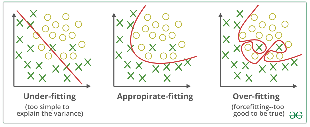
# Generalization Error
📗 With a large number of hidden layers and units, a neural network can overfit a training set perfectly. This does not imply the performance on new items will be good: Wikipedia.
➩ More data can be created for training using generative models or unsupervised learning techniques.
➩ A validation set can be used (similar to pruning for decision trees) to train the network until the loss (or accuracy) on the validation set begins to increase.
➩ Dropout can be used: randomly omitting units (random pruning of weights) during training so the rest of the units will have a better performance: Wikipedia.
Example
# Regularization
📗 A simpler model (with fewer weights, or many weights set to 0) is usually more generalizable and would not overfit the training set as much. A way to achieve that is to include an additional cost for non-zero weights during training. This is called regularization: Wikipedia.
➩ \(L_{1}\) regularization adds \(L_{1}\) norm of the weights and biases to the loss, or \(C = C_{1} + C_{2} + ... + C_{n} + \lambda \left\|\begin{bmatrix} w \\ b \end{bmatrix}\right\|_{1}\), for example, if there are no hidden layers, \(\left\|\begin{bmatrix} w \\ b \end{bmatrix}\right\|_{1} = \left| w_{1} \right| + \left| w_{2} \right| + ... + \left| w_{m} \right| + \left| b \right|\). Linear regression with \(L_{1}\) regularization is also called LASSO (Least Absolute Shrinkage and Selector Operator): Wikipedia.
➩ \(L_{2}\) regularization adds \(L_{2}\) norm of the weights and biases to the loss, or \(C = C_{1} + C_{2} + ... + C_{n} + \lambda \left\|\begin{bmatrix} w \\ b \end{bmatrix}\right\|^{2}_{2}\), for example, if there are no hidden layers, \(\left\|\begin{bmatrix} w \\ b \end{bmatrix}\right\|^{2}_{2} = \left(w_{1}\right)^{2} + \left(w_{2}\right)^{2} + ... + \left(w_{m}\right)^{2} + \left(b\right)^{2}\). Linear regression with \(L_{2}\) regularization is also called ridge regression: Wikipedia.
📗 \(\lambda\) is chosen as the trade-off between the loss from incorrect prediction and the loss from non-zero weights.
➩ \(L_{1}\) regularization often leads to more weights that are exactly \(0\), which is useful for feature selection.
➩ \(L_{2}\) regularization is easier for gradient descent since it is differentiable.
➩ Try \(L_{1}\) vs \(L_{2}\) regularization here: Link.
In-class Discussion
📗 [1 points] Fix some \(d\), find the point where \(\left\|\begin{bmatrix} w_{1} \\ w_{2} \end{bmatrix}\right\| \leq d\) and minimize the cost \(c\). Use regularization.
➩ Aside: compare the above procedure with: fix some cost \(c\), find the point with the minimum distance to the origin \(d\). This is related to this duality of optimization.
Bound \(d\): 0.5
Cost \(C\): 0
1 slider
[Q2]
# Questions?
📗 If you have questions, please use (i) Zoom chat, (ii) Piazza: Link, (iii) Office hours and discussion sessions. Please do NOT use Canvas mail and use email only to the course instructor (not TAs) for grading issues.
Additional In-class Discussion
📗 Sometimes a question not in the notes will be asked during the lecture, you can submit your answer here:
Notes (not visible to other students):
[Q3]
Submit your answer to see other students answers (click the submit button to refresh):
Additional In-class Quiz
📗 Sometimes a question not in the notes will be asked during the lecture, you can submit your answer here:
A. B.
C.
D.
E.
Notes (not visible to other students):
[Q4]
Submit your answer to see other students answers (click the submit button to refresh):
test nnd,sgd,sfm,rd q https://script.google.com/macros/s/AKfycbyiidUAdiLc3YrKgOAM6T95ATulwDQxQilWVv1bK1L5sKRl8ozXfVs4PjCC2VtMWcIBpg/exec
# In-class Quiz Instructions
📗 To get full points on the in-class quizzes for a lecture:
➩ Submit relevant answers to the questions discussed during the lecture: incorrect answers are okay.
➩ Some questions require [notes] to earn the point.
➩ Some questions require special ID (given during the lecture) to earn the point.
➩ Do not submit answers to questions that are not discussed during the lectures. Each such submission will result in a deduction of one point.
➩ Submissions after the lecture, before the midterm (first 14 lectures) and the final exam (last 14 lectures), are accepted. After the exams, no in-class quiz submissions will be accepted.
➩ The grade on Canvas Assignment Q4 is computed as number of points divided by the number of questions asked (out of 1) and updated on Canvas every weekend.
📗 If there are any issues with submission on the website, please use this Google form: Link.
📗 Bonus point opportunities during a few lectures (added to in-class quiz above 20 points).
📗 Notes and code adapted from the course taught by Professors Jerry Zhu, Blerina Gkotse, Yudong Chen, Yingyu Liang, Charles Dyer. Some content are generated using Copilot .
Prev: L3, Next: L5
Last Updated: July 16, 2026 at 12:17 PM