Prev: L6, Next: L8
Zoom: Link, Piazza: Link, Google Form: Link.
Wisc ID for in-class quiz: (if your wisc email is "test@wisc.edu", please enter "test")
Token: (will be given during the lectures)
7
id,answer_id;token,answer_check
Slide:
# K Nearest Neighbor
📗 K Nearest Neighbor algorithm (not related to K Means) is a simple supervised learning algorithm that uses the \(K\) items from the training set that is the closest to a new item to predict the label of the new item: Link, Wikipedia.
➩ 1 nearest neighbor copies the label of the closest item.
➩ 3 nearest neighbor finds the majority label of the three closest items.
➩ N nearest neighbor uses the majority label of the training set (of size N) to predict the label of every new item.
📗 The distance measure used in K nearest neighbor can be any of the \(L_{p}\) distances.
➩ \(L_{1}\) Manhattan distance.
➩ \(L_{2}\) Euclidean distance.
➩ \(L_{\infty}\) Maximum distance from all features.
In-class Discussion
ID:📗 [1 points] Find the value of K for K nearest neighbor that is the most appropriate for the dataset. Click on an existing point to perform leave-one-out cross validation, and click on a new point to find the nearest neighbor.
K:
[Q1]
# Training Set Accuracy
📗 For 1NN, the accuracy of the prediction on the training set is always 100 percent.
📗 When comparing the accuracy of KNN for different values of K (called hyperparameter tuning), training set accuracy is not a great meausre.
📗 K fold cross validation is often used instead to measure the performance of a supervised learning algorithm on the training set.
➩ The training set is divided into K groups (K can be different from the K in KNN).
➩ Train the model on K - 1 groups and compute the accuracy on the remaining 1 group.
➩ Repeat this process K times.
📗 K fold cross validation with \(K = n\) is called Leave One Out Cross Validation (LOOCV).
In-class Quiz
ID:📗 [4 points] Given the following training data, what is the fold cross validation accuracy if NN (Nearest Neighbor) classifier with Manhattan distance is used. The first fold is the first instances, the second fold is the next instances, etc. Break the tie (in distance) by using the instance with the smaller index. Enter a number between 0 and 1.
| \(x_{i}\) | ||||||
| \(y_{i}\) |
📗 Answer: .
[Q2]
Other students' answers:
# Computer Vision Tasks
📗 Unsupervised:
➩ Image segmentation.
📗 Supervised:
➩ Image colorization.
➩ Image reconstruction.
➩ Image synthesis.
➩ Image captioning.
➩ Object detection and tracking.
➩ Medical image analysis.
# Convolution
📗 Pixels are not independent of their neighbors. Ignoring the dependence is inappropriate for most computer vision tasks.
📗 Neighboring pixel intensities can be combined to create one feature that captures the information in the region around the pixel.
📗 Linearly combining pixels in a rectangular region is called convolution: Wikipedia.
➩ The convolution of an \(m \times m\) matrix (representing a training image indexed \(i\)) \(X_{i}\) with a \(\left(2 k + 1\right) \times \left(2 k + 1\right)\) filter \(W = \left[W_{s t}\right]_{s = -k, ..., k, t = -k, ..., k}\) is an \(m \times m\) matrix \(A_{i} = X_{i} \star W\), where the row \(r\) column \(c\) entry is given by \(\left[A_{i}\right]_{r c} = \displaystyle\sum_{s = -k}^{k} \displaystyle\sum_{t = -k}^{k} \left[X_{i}\right]_{r + t, c + s} W_{-s, -t}\).
➩ Technical note: the definition here flips the filter, for example the filter \(\begin{bmatrix} 1 & 2 & 3 \\ 4 & 5 & 6 \\ 7 & 8 & 9 \end{bmatrix}\) is flipped to \(\begin{bmatrix} 9 & 8 & 7 \\ 6 & 5 & 4 \\ 3 & 2 & 1 \end{bmatrix}\) before linear combination with the image. Similar linear combination without flipping the filter is called cross-correlation.
➩ The convolution filter is also called "kernel", but different from the kernel matrix for SVMs.
Math Note
📗 Convolution between two 1D vectors is also defined: the convolution of a vector \(x_{i} = \left(x_{i 1}, x_{i 2}, ..., x_{i m}\right)\) with a filter \(w = \left(w_{-k}, w_{-k + 1}, ..., w_{k-1}, w_{k}\right)\) is: \(a_{i} = \left(a_{i 1}, a_{i 2}, ..., a_{i m}\right) = x \star w\), where \(a_{i j} = w_{-k} x_{i \left(j + k\right)} + w_{-k + 1} x_{i \left(j + k - 1\right)} + ... + w_{k} x_{i \left(j - k\right)}\) for \(j = 1, 2, ..., m\).
📗 3D convolution can be defined in a similar way.
Example
In-class Discussion
📗 [1 points] Upload an image and try one of the following filters: . Image:
![]() 1. Click on the image to perform convolution with this filter: .
1. Click on the image to perform convolution with this filter: .
For Gaussian filter: size = , \(\sigma\) = . 0
[Q3]
In-class Quiz
ID:📗 [4 points] What is the convolution between the image and the filter using zero padding? Remember to flip the filter first.
📗 Answer (matrix with multiple lines, each line is a comma separated vector): .
[Q4]
Other students' answers:
# Traditional Computer Vision
📗 Traditional computer vision algorithms use engineered features for images based on image gradients.
➩ Image gradients are changes in pixel intensity due to the change in the location of the pixel: Wikipedia.
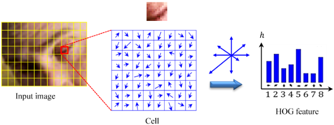
➩ Histogram of Gradients (HOG) can be used as a features for images and is often combined with SVM for face detection and recognition tasks: Wikipedia.
Math Note
📗 Image gradients can be computed (approximated) by convolution with the following filters: \(\nabla_{x} I = W_{x} \star I\) and \(\nabla_{y} I = W_{y} \star I\).
➩ (Discrete) derivative filter: \(W_{x} = \begin{bmatrix} -1 & 0 & 1 \\ -1 & 0 & 1 \\ -1 & 0 & 1 \end{bmatrix}\) and \(W_{y} = \begin{bmatrix} -1 & -1 & -1 \\ 0 & 0 & 0 \\ 1 & 1 & 1 \end{bmatrix}\).
➩ Sobel filters: \(W_{x} = \begin{bmatrix} -1 & 0 & 1 \\ -2 & 0 & 2 \\ -1 & 0 & 1 \end{bmatrix}\) and \(W_{y} = \begin{bmatrix} -1 & -2 & -1 \\ 0 & 0 & 0 \\ 1 & 2 & 1 \end{bmatrix}\), which can be viewed as a combination of the Gaussian filter (to blur the image) and the derivative filter: Wikipedia.
📗 Gradient magnitude at a pixel \((s, t)\) is given by \(G = \sqrt{\nabla_{x}^{2} I\left(s, t\right) + \nabla_{y}^{2} I\left(s, t\right)}\) and gradient direction \(\Theta = arctan\left(\dfrac{\nabla_{y} I\left(s, t\right)}{\nabla_{x} I\left(s, t\right)}\right)\).
Math Note
📗 For HOG features: in every 8 by 8 pixel region of an image, the gradient vectors \(\begin{bmatrix} \nabla_{x} I\left(s, t\right) \\ \nabla_{y} I\left(s, t\right) \end{bmatrix}\) are put into 9 orientation bins, for example, \(\left[0, \dfrac{2}{9} \pi\right], \left[\dfrac{2}{9} \pi, \dfrac{4}{9} \pi\right], ..., \left[\dfrac{16}{9} \pi, 2 \pi\right]\), and the histogram count is used as the HOG features.
📗 The resulting bins are normalized within a block of 2 by 2 regions.
📗 Scale Invariant Feature Transform (SIFT) produces similar feature representation using histogram of oriented gradients: Wikipedia.
➩ It is location invariant.
➩ It is scale invariant: images at different scales are used to compute the features.
➩ It is orientation invariant: dominant orientation in a larger region is calculated and all gradients in the region are rotated by the dominant orientation.
➩ It is illumination and contrast invariant: feature vectors are normalized so that they sum up to 1, and thresholded (values smaller than a threshold, for example 0.2, are made 0).
In-class Discussion
ID:📗 [1 points] Select the pixels in each of the 9 bins. The histogram is computed by summing up the .
1 0
# Haar Features
📗 HOG and SIFT features are too expensive to compute for real-time face detection tasks.
📗 Each image contains large number of locations at different scales, but faces only occur in very few of them.
📗 Each feature and classifier based on the feature should be easy to compute, and boosting can be used to combine simple features and classifiers.
📗 Haar features are differences between sums of pixel intensities in rectangular regions and can be obtained by convolution with filters such as \(\begin{bmatrix} 1 & 1 \\ -1 & -1 \end{bmatrix}\), \(\begin{bmatrix} 1 & -1 \\ 1 & -1 \end{bmatrix}\), ...: Wikipedia.
📗 Integral images (sum of pixel intensities above and to the left of every pixel) can be used to further speed up the computation: Wikipedia.
# Cascade Classifiers
📗 Each weak classifier can be a decision stump (decision tree with only one split) based on a Haar feature.
📗 Finding the threshold by comparing information gain is computationally expensive, so it is usually computed as the mid-point of the averages of the two classes.
📗 A sequence of weak classifiers can be combined into a strong classifier using AdaBoost (Adaptive Boosting).
➩ Start with a weak classifier and equal weights on all training items.
➩ Increase the weights on the items that are classified incorrectly, and train another weak classifier based on the updated weights.
➩ Continue the process to create a sequence of weak classifiers. The combined classifier is called a strong classifier.
📗 A sequence of strong classifiers can be combined into a cascade classifier.
➩ Start with a classifier with close to 100 percent detection rate by a possibly large false-positive rate.
➩ Train the next classifier still with close to 100 percent detection rate but with lower false-positive rate.
➩ Repeat this process to get a sequence of classifiers. The combined classifier called a cascade classifier.
Math Notes
📗 To create each classifier in the cascade classifier:
➩ Start by assigning equal weights for each image: \(w_{i} = \dfrac{1}{n}\) for \(i = 1, 2, ..., n\).
➩ Find optimal feature and threshold given the weights: the cost of mistake on image \(i\) should be weighted by \(w_{i}\), for example, \(C = C_{1} + C_{2} + ... + C_{n}\) where \(C_{i} = w_{i}\) if \(f_{j}\left(x_{i}\right) = y_{i}\) and \(C_{i} = 0\) otherwise.
➩ Choose weight of classifier \(f_{j}\) to be \(\alpha_{j} = \dfrac{1}{2} \log\left(\dfrac{1 - C}{C}\right)\).
➩ Update the weights to \(w_{i} = w_{i} \cdot e^{-y_{i} \alpha_{j} f_{j}\left(x_{i}\right)}\).
➩ Repeat the process until the desired detection rate and false positive rates are reached: the resulting classifier is \(\alpha_{1} f_{1} + \alpha_{2} f_{2} + ...\).
Example
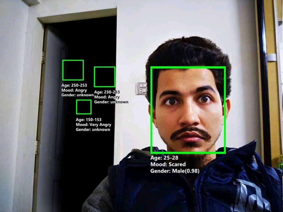
# Viola Jones
📗 Viola Jones algorithm is a popular real-time face detection algorithm: Wikipedia.
➩ Each classifier operates on a 24 by 24 region of the image at multiple scales (scaling factor of 1.25).
➩ The regions can be overlapping. Nearby detection of faces are combined into a single detection.
# Questions?
📗 If you have questions, please use (i) Zoom chat, (ii) Piazza: Link, (iii) Office hours and discussion sessions. Please do NOT use Canvas mail and use email only to the course instructor (not TAs) for grading issues.
Additional In-class Discussion
📗 Sometimes a question not in the notes will be asked during the lecture, you can submit your answer here:
Notes (not visible to other students):
[Q6]
Submit your answer to see other students answers (click the submit button to refresh):
Additional In-class Quiz
📗 Sometimes a question not in the notes will be asked during the lecture, you can submit your answer here:
A. B.
C.
D.
E.
Notes (not visible to other students):
[Q7]
Submit your answer to see other students answers (click the submit button to refresh):
test kn,cv,fil,cnv,hog q https://script.google.com/macros/s/AKfycbyiidUAdiLc3YrKgOAM6T95ATulwDQxQilWVv1bK1L5sKRl8ozXfVs4PjCC2VtMWcIBpg/exec
# In-class Quiz Instructions
📗 To get full points on the in-class quizzes for a lecture:
➩ Submit relevant answers to the questions discussed during the lecture: incorrect answers are okay.
➩ Some questions require [notes] to earn the point.
➩ Some questions require special ID (given during the lecture) to earn the point.
➩ Do not submit answers to questions that are not discussed during the lectures. Each such submission will result in a deduction of one point.
➩ Submissions after the lecture, before the midterm (first 14 lectures) and the final exam (last 14 lectures), are accepted. After the exams, no in-class quiz submissions will be accepted.
➩ The grade on Canvas Assignment Q7 is computed as number of points divided by the number of questions asked (out of 1) and updated on Canvas every weekend.
📗 If there are any issues with submission on the website, please use this Google form: Link.
📗 Bonus point opportunities during a few lectures (added to in-class quiz above 20 points).
📗 Notes and code adapted from the course taught by Professors Jerry Zhu, Blerina Gkotse, Yudong Chen, Yingyu Liang, Charles Dyer. Some content are generated using Copilot .
Prev: L6, Next: L8
Last Updated: July 16, 2026 at 12:17 PM