Examples:
Demonstrate Newton's Method graphically for the following function:
 .
.
Hint: Print a plot of the function between 0 and 0.5 and mark each successive root approximation with a line tangent to the function at that point to get the next approximation.
Newton's Method can be demonstrated graphically as follows for the function
.
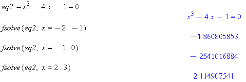
1 Plot the function to see approximately where the root lies and make an initial guess. (We can see that the actual root is larger than 0.2, but we wish to illustrate the algorithm and it is easier to see if we start a little farther away.) 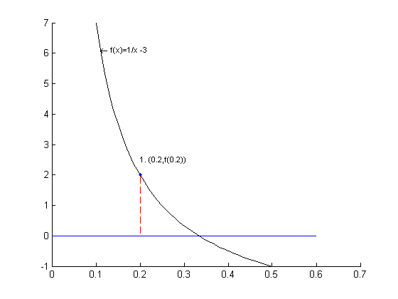
2 Mark the point (0.2,f(0.2)) and draw a line tangent to the curve at this point. Record where the tangent line crosses the x-axis. In this case, the tangent line crosses the x-axis at 0.28. 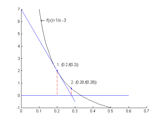
3 Repeat the approximation steps for the new approximation value. Mark the point (0.28,f(0.28)) and draw the line tangent to the curve at the point (0.28,f(0.28)). Record where this new tangent line crosses the x-axis. This time is at x.0.3248. 
4 Repeat to find the next approximation(s) until you find as accurate an approximation as you need for your particular problem. 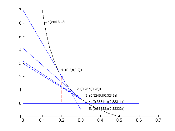
This algorithm will produce successive values of x (the root of the equation) that are closer and closer to the exact solution. And equally important, the error in successive steps is reduced substantially.
- Compare the percentage error of each successive approximation to see how quickly Newton's method converges to the actual value. The percentage error is the (difference between the approximate value and the exact value) divided by the exact value and multiplied by 100.
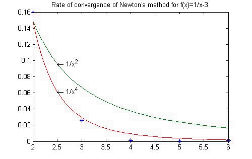
Note how quickly the approximations converge. This rate is known as the rate of convergence and is a useful measure for comparing numeric algorithms.
Iteration Number x Error % Error 0 0.2 0.133333333333333 40% 1 0.28 0.053333333333333 16% 2 0.3248 0.008533333333333 2.56% 3 0.33311488 0.000218453333333 0.065536% 4 0.333333190167757 0.000000143165577 0.0000429% 5 0.333333333333272 0.000000000000061 1.8435e-11% 6 0.333333333333333 -0.000000000000000 -1.7e-14% 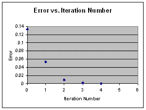
Find the roots of the polynomial equation
 and as a decimal out to 7 decimal points using Newton's Method.
The roots are clearly
 . These are not rational numbers (i.e. they cannot be expressed as the ratio of integers). Therefore Newton’s Method must be used to determine the root value up to a specified accuracy. Most computer hardware works with 17 decimal digits of precision so it is senseless to compute more than 17 digits of accuracy. Using the Newton’s Method formula on this function gives
 and
and
 thus
thus

So the formula is

Choose an initial guess of
 and use the successive approximation process.
# 

0 1 1.5 1 1.5 1.416667 2 1.416667 1.414215 3 1.414215 1.414213 4 1.414213 1.414213 In only 4 steps Newton’s Method has computed the value of
 up to 7 digits of accuracy. Notice that the positive root was found. This is because the initial guess was “closest” to this root and the function monotonically increased toward this root. To find the other negative root you must make an initial guess where the function monotonically increases or decreases toward that root. Either
 or
or
 would work.
Find the roots of the polynomial equation
 using Newton's Method.
The values of the roots of this equation are not so obvious. Since Newton’s Method requires you to make an intelligent first guess (i.e. the function must monotonically approach a root from the initial
 ) you should plot the function first to see where the roots are.
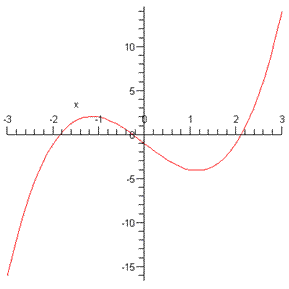
From this plot you see that initial guesses of
=-2,
=0, and
=2 will each be close to the three roots. Now you obtain the formula that you will use to successively approximate the roots.

#
0 2 2.125 1 2.125 2.114975 2 2.114975 2.114907 3 2.114907 2.114907 0 0 -0.25 1 -0.25 -0.2704918 2 -0.2704918 -0.2540451 3 -0.2540451 -0.2541016 4 -0.2541016 -0.2541016 0 -2 -1.875 1 -1.875 -1.860978 2 -1.860978 -1.860805 3 -1.860805 -1.860805 Check your answers using the Maple
fsolvecommand.