CS 766 Project 4 - Uncalibrated Stereo Vision

Results

We discuss here our results from the various stages of the pipe-line. From the overview, the steps are:

0 - Find Correspondence using the KLT feature point tracker.
1 - Determine the Fundamental Matrix, F.
2 - Recify images using F.
3 - Apply Birchfield and Tomasi calibated stereo correspondence algorithm to create a depth map.
4 - If the depth map generated is bad, determine new correspondence points by searching the space near the epipolar lines determine originally.
5 - Repeat from step 1, using the new correspondence points.

Step 0 - Find Correspondence using the KLT feature point tracker

Though KLT is sufficiently good at finding features, the tracker did not perform well for our purposes. We tried a number of the following methods for finding better correspondences given KLT output:

Ignore tracking data and run RANSAC to find a fundamental matrix that is consitent. That is, that each feature in one image has another feature in the other image that lies near the epipolar line. Unfortunately, since it is highly probable that some feature will lie near a given epipolar line, this also has poor results.
Like #1, use RANSAC, but only score how close a feature that KLT succesfully tracked is to the epipolar lines. Again, this gave poor results, since a few poorly tracked features would score well.
Again using RANSAC, find the best fundamental matrix that is internally consistent. That is, do not score using all features, or all tracked features, but only those used to determine the fundamental matrix in the first place. In this case, use more than 8 points for calculating F, so that F is simply an approximation to those points. Again, a few bad correspondences appear in well scoring sets.
A method proposed by M. Pilu. This method first generates a pairwise proximity matrix between all features, using pixel position and a local normalized cross correlation. The SVD of this matrix is taken, and the diagonal values are set to 1. Once multiplied back together, we are given a scoring matrix between pairwise correspondences. Pilu uses this matrix to find correspondences between all pairs, however we are only interested in a few, best correspondences. We therefore pick the best N scoring correspondences to use for tracking.

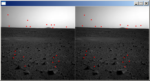
Good correspondences tend not to be well distributed throughout the image. This increases the error in later steps, since the determined fundamental matrix tends to be inaccurate for finding epipolar lines far from the tracked features. To avoid this, we split the image into fourths, and run tracking and correspondence on each smaller image. This distributes the correspondences while still giving us good matches.

Note that this will still produce bad results in regions where poor features have been detected as seen in the sky of this pair of mars images.

Step 1 Determine the Fundamental Matrix, F
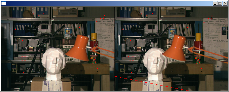
OpenCV provides a method for this calculation. A good discussion of the 8-point algorithm is given by Hartley. Note that this calculation is very much sensitive to noise. For example, the following image is a parallel stereo pair. In other words, all epipolar lines should be horizontal. Note that almost all points are tracked reasonably, however if we examine the epipolar line that corresponds to the top-left of the box (white square), it is not horizontal and misses the point in the corresponding image.

The calculated fundamental matrix provides much better results in other parts of the image

Step 3 - Apply Birchfield and Tomasi calibated stereo correspondence algorithm to create a depth map
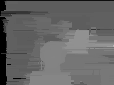
Birchfield and Tomasi use a dynamic programming method to determine disparity given two rectified images. Essentially, they perform a global sequence alignment between each pair of lines. This method is provided by openCV. Perfectly rectified images give the depth image below. This image has been brightness enhanced.