Examples:
Use the same worksheet (without
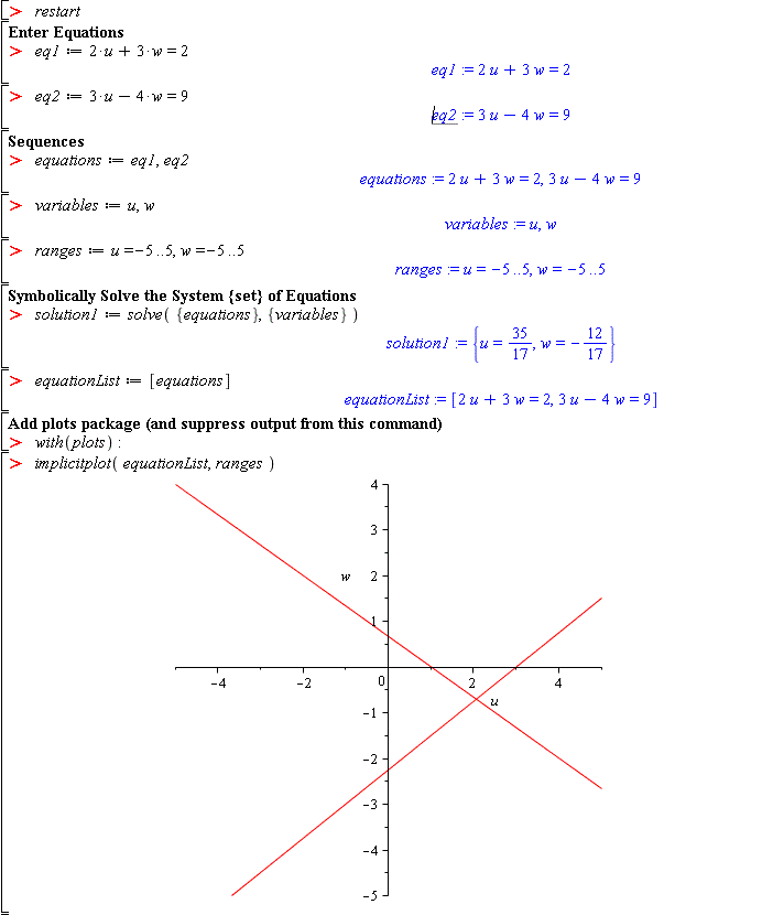
restartfor all of the exercises and pay attention to the results of each command statement. To be able to use Maple effectively, students must understand which commands require expressions, equations, values, etc. It is also necessary to understand the result of each command.Solve two equations for two unknowns using a single solve command as shown here. Note that when a set of multiple equations is solved for its set of multiple variables, the symbolic result is a set of equations: one for each variable.
        eq1 := 2*u + 3*w = 2
        eq2 := 3*u - 4*w = 9
        equations := eq1,eq2
        variables := u,w
        ranges := u=-5..5, w=-5..5
        solution1 := solve( {equations} , {variables} )
        equationList := [equations]
        with(plots): implicitplot(equationList, ranges)
Comment: Notice how only one
solvecommand is needed to solve for both unknowns. This is because we have solved the linear system and each equation is needed to solve for each unknown. It is a mistake to try and solve the equations separately and then somehow combine the results. Make sure that you understand to solve a system of equations as a system (set) of equations.Also note how the solution is displayed as a set since the order of u and w do not matter. The plot of the two lines shows how the solution corresponds to the (u,w) point of intersection. Final comment, the unknowns do not need to be x,y. They can be any variables that you want.
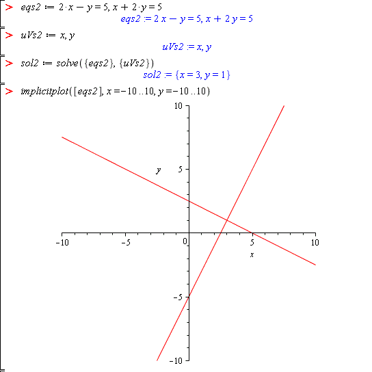
          eqs2 := 2*x - y = 5, x + 2*y = 5
          uVs2 := x, y
          sol2 := solve({eqs2}, {uVs2})
          implicitplot([eqs2], x=-10..10, y=-10..10)
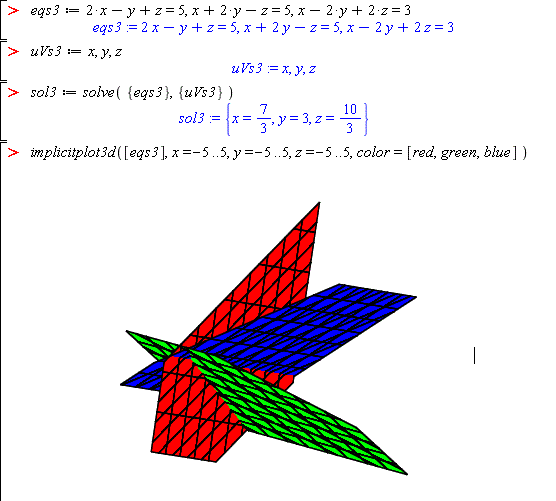
        eqs3 := 2*x - y + z = 5, x + 2*y - z = 5, x - 2*y + 2*z = 3
        uVs3 := x, y, z
        sol3 := solve({eqs3}, {uVs3})
        implicitplot3d([eqs3], x=-5..5,y=-5..5, z=-5..5)
Comment: The geometric interpretation of the solutions of sets of two and three linear equations as the intersection of two lines or three planes is useful from a conceptual point of view. However it is limited to a maximum of three equations and three unknowns. How can we display four dimensions? Four equations and four unknowns does not have a geometric interpretation, however the general concept is the same. (The plot has been turned slightly to better show the intersection point)
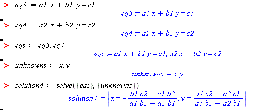
          eq3 := a1*x + b1*y = c1
          eq4 := a2*x + b2*y = c2
          eqs := eq3,eq4
          unknowns := x,y
          solution4 := solve({eqs},{unknowns})
Comment: Note that Maple really does solve these equations symbolically. The solution in the case of generic coefficients is formulas in terms of the coefficients.
          eq5 := a1*x + b1*y + c1*z = d1
          eq6 := a2*x + b2*y + c2*z = d2
          eq7 := a3*x + b3*y + c3*z = d3
          eq567 := {eq5,eq6,eq7}
          unknownsxyz := {x,y,z}
          solutionxyz := solve(eq567,unknownsxyz)
Comment: Maple will solve equations with generic coefficients of arbitrarily large complexity, but at some point it is not practical to solve problems in this way. However, it is usually practical to solve systems of equations with numeric coefficients.

