Examples:

1. eq1 := x + 2*y = 3
eq2 := (x+1)^2 – 2y = 2
solve({eq1,eq2},{x,y})
with(plots):
implicitplot([eq1,eq2], x=-5..5, y=-5..5)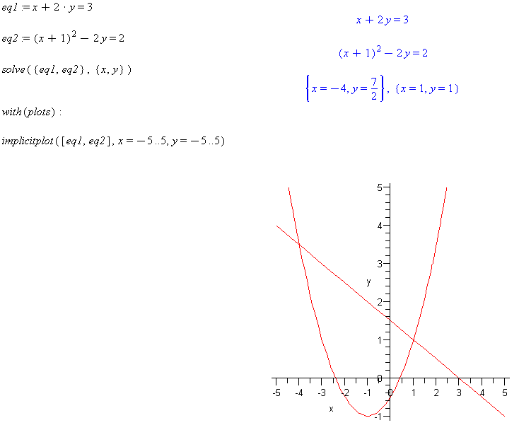
   

   Comment: Note that there are two solution (x,y) points. The plot shows that the line corresponding to the linear equation intersects the parabola at two points.

2. eq3 := x^2-y=4
eq4 := -2*x^2-y=-23
with(plots):
implicitplot([eq3, eq4], x=-4..4, y=-10..10)
sol34 := solve({eq3, eq4}, {x, y})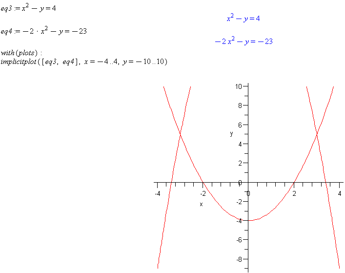

   

   Comment: Note that Maple was able to find the intersection points of these two parabolas, both equations being non-linear.

3. eq5 := y^2=x+2
eq6 := y=x
with(plots):
implicitplot([eq5, eq6], x=-10..10, y=-10..10)
sol56 := solve({eq5, eq6}, {x, y})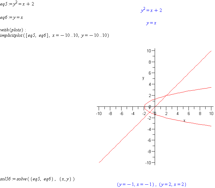

   

   Comment: Note that Maple solves for the roots of multi-valued functions like the first in this set.

4. eq7 := y=x^2
eq8 := y=x+4
with(plots):
implicitplot([eq7, eq8], x=-10..10, y=-5..100)
sol78 := solve({eq7, eq8}, {x, y})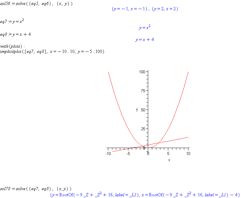

   

   Comment: The result returned by Maple does not look like a solution and contains RootOf in the result. This means that Maple has created this intermediate result and is asking if it could possibly be true that you are seeking more than one root. Respond by typing the command allvalues(sol78). Maple will then return the two roots. Always try the allvalues(name) command when you see RootOf in the result generated by Maple. This will usually complete the solution of the problem.

   

5. eq9 := y=ln(x)
eq10 := y-3=-2*x
with(plots):
implicitplot([eq9, eq10], x=-3.5..10, y=-10..10)
sol910 := solve({eq9, eq10}, {x, y})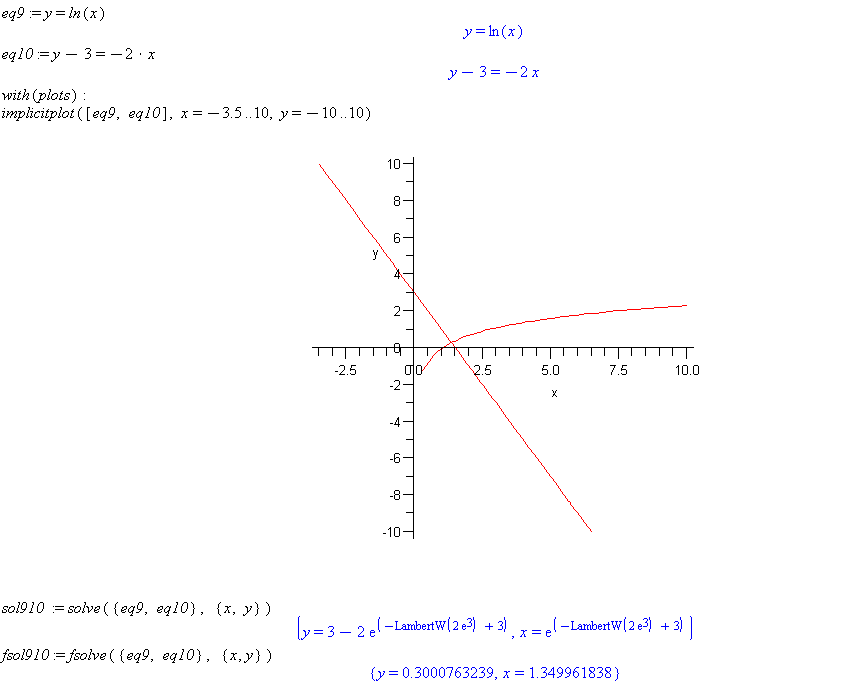

   

   Comment: The solve command fails to return a solution to this system of equations that includes a non-linear equation involving the logarithm. Use fsolve({eq9, eq10}, {x, y}) to get a decimal value.

6. eq11 := y^2=ln(x)
eq12 := y+3=2*x
with(plots):
implicitplot([eq11, eq12], x=-3.5..10, y=-10..10)
sol1112 := solve({eq11, eq12}, {x, y})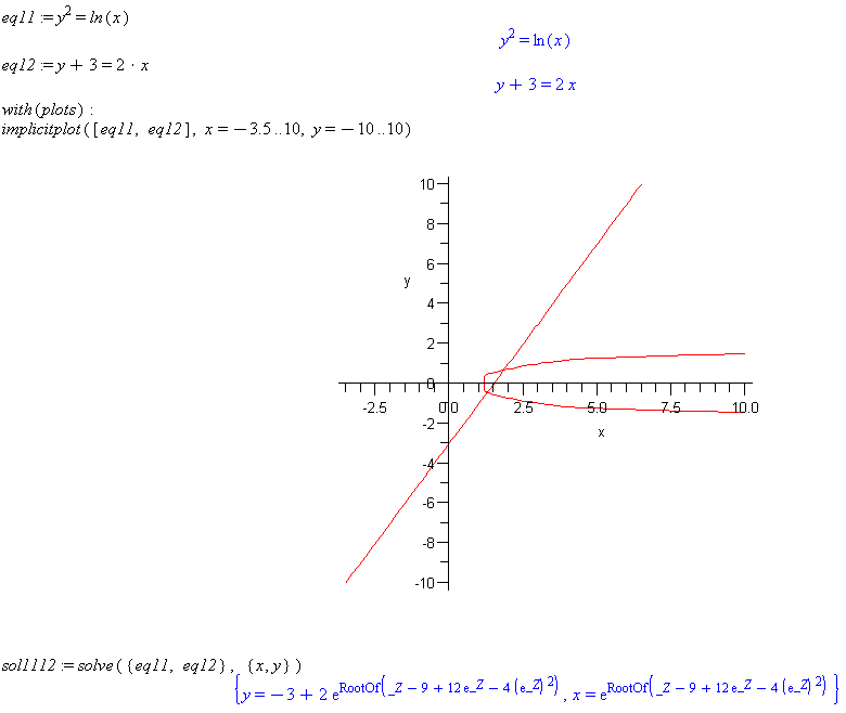

   

   Comment: The solve command fails to give a result. This set of equations will have to be solved numerically. See the next example.

7. nonlinearEqs:= {y^2=ln(x), y+3=2*x}
fsolve(nonlinearEqs, {x,y}, x=1..1.5, y=-2..0)
fsolve(nonlinearEqs, {x,y}, x=1.5..2, y=0..2)

   

   Comment: The first execution of fsolve finds the root below the x-axis and the second execution finds the root above the x-axis by specifying ranges of x and y that bracket that particular root.