Getting Started
Create a new script (m-file) in MATLAB and add a clear command to the top of your script.
Problem 1: Charging an RC Circuit
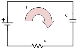
A simple RC circuit with a battery is shown below:
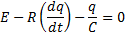
The circuit consists of a battery, resistor (R), and capacitor (C) connected in a series. Suppose that the capacitor is initially uncharged and then a battery is connected. We will denote the time (t) the battery is connected as time t = 0. Initially, the potential difference across the resistor is the battery emf but then steadily drops. Applying Kirchoff's law, we get

where E is the emf of the battery, I is the current (so IR is the voltage drop across the resistor), q is the magnitude of the charge on the capacitor plates, and q/C is the voltage difference across the plates. Since the current is the rate of change of the charge, we can rewrite this equation as:
At time 0, the initial value of q is 0.
Note: although this equation can be solved analytically, it is a good ODE to demonstrate the use of MATLAB's ode45() function.
Solve for the steady-state (by hand). Note that your answer will contain symbolic constants.
Write a function, called circuitODE, that computes the value of the derivative of q(t). The function must take as input the parameters t and q (in that order) and return the derivative of q(t) using the equation above. Hint: solve for dq/dt first and then you may evaluate the value of that derivative for any value of t and q desired. For this and many such problems, t is not needed to compute the derivative, but in general the time is needed, so it is always included. The first line of your circuitODE.m file should look like
function qprime = circuitODE(t, q)
Use the values R = 8.0×10³ Ω, C = 2.0×10⁻⁶ F, and E = 1.5 V
Add code to your teamLab14 script to call ode45() and plot the solution as potential across capacitor ( = q/C) vs time. In the main program you should set the conditions defining the solution such as the initial value of q, the initial time, and the time interval over which the ODE is to be solved. Compute the solution from time equals 0 to 0.05 seconds. Once the argument variables have been initialized, your call to ode45 should look like
[t_soln, q_soln] = ode45(@circuitODE, timespan, q0);
What is the potential across the capacitor at 0.05 seconds?
From the plot of the potential across the capacitor, it is apparent that there is a limit. What is the value of this limit? (You may want to change the timespan over which you solve the ODE.) How does this compare to what you determined in part a?
Show the plot figures and your answers to parts c and d to a lab leader.
Problem 2: Motion of a Pendulum
A classic problem in physics is the oscillatory motion of a pendulum as shown in the figure below.
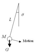
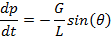
The equation that governs the motion of the pendulum is:
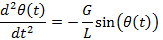
The force of gravity is in the downward direction and the acceleration is expressed as the angular acceleration. This second-order ordinary differential equation requires two initial conditions, one for θ and one for its first derivative dθ/dt. The initial conditions we will use are θ(0)=θ0 and dθ(0)/dt = 0, where θ0 is the initial position of the pendulum in radians. The length of our pendulum, L, is 2 meters.
This is a non-linear ODE because sin(θ) appears on the right hand side. This equation requires a numerical solution. Since we have a second-order ODE, we will first convert the single second-order ODE into a system of two first-order ODEs. We define a new variable p = dθ/dt and re-write our second-order ODE as two first-order ODES:
Write a function, called pendODE, whose first line looks like
function wprime = pendODE(t, w)
where w is a vector with two parts (i.e., w is of the form [theta, p]) and the function computes a vector of derivatives wprime (where wprime = [thetaprime; pprime] ← note the use of ;). (Note that G = 9.8 m/s2 and L = 2 m)
Add code to your teamLab14 script to solve the non-linear ODE for the pendulum motion using ode45 over the time span 0 to 6π with initial conditions θ0 = π/10 radians and dθ(0)/dt = 0. Plot the solution for θ(t).
The usual approach in elementary physics courses is to make the small amplitude approximation that for small angles θ, sin(θ) ≈ θ. This produces an approximate equation that is nearly correct for small amplitudes. The approximate equation is:
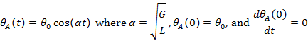
This is an ODE that can be solved symbolically (see the example from lecture, p. 5); the solution is:
This very simple result is the basis for a huge part of classical physics since it represents the essence of the harmonic oscillator problem where motion is governed by a restoring force. However it is important to recognize that this approximate equation is only valid for small values of θ.
We now compare the numeric solution for the non-linear ODE to the results that use the small amplitude approximation.
Add commands to your teamLab14 script that compute θA(t) for the small amplitude approximation, θA(t) = θ0 cos(αt) for the same values of t for which the exact solution was computed using ode45 in part 2.b
Compare the ode45 solution to the small amplitude result by plotting both (on the same plot figure) for the case θ0 = π/10.
Compare the two solutions for
Does the solution to the exact non-linear ordinary differential equation still look like the solution to the approximate linearized version? At what initial amplitude do the solutions begin to differ? Which one is in error?
Show your results to a lab leader.
The motion of a damped spring-mass system can be described using the following 2nd-order ODE:
m x'' (t) + c x' (t) + k x(t) = 0
where x indicates the displacement from the equilibrium position (m), t is the time (s), m is the mass (kg), c is a damping coefficient (N·s/m), and k is a spring constant (N/m). Suppose m = 20 kg and k = 20 N/m. Solve this ODE for t from 0 to 15 seconds with initial conditions x(0) = 1 m and x' (0) = 0 m/s and plot the results for each of the following situations:
Hint: Convert the second-order ODE to a system of first-order ODEs.