CS524 - Intro to Optimization | Iván Jaen Márquez

Introduction

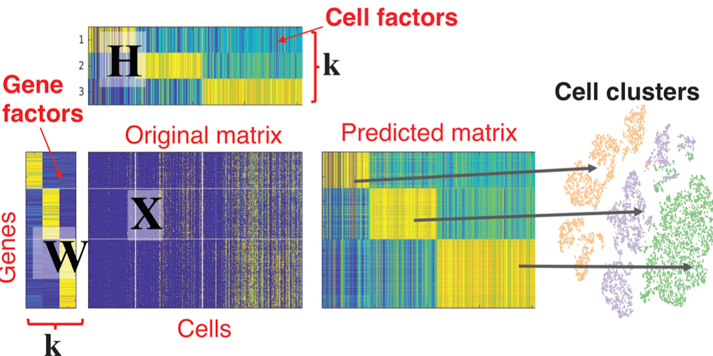
Non-negative Matrix Factorization (NMF) is an unsupervised learning technique that allows to approximate a high-dimensional non-negative matrix \(X\) (all entries are \(X_{ij}>0\)) into two non-negative low rank matrices \(W\), \(H\) of rank \(k<<min(m,n)\). In the context of gene expression matrices, the rows of \(X\) correspond to genes, and columns correspond to cells. NMF factorizes the gene expression matrix into a:

Gene signature matrix (\(W\))

Contains a set of gene expression patterns or modules, which represent the co-expression of genes across multiple samples.
Cell coefficient matrix (\(H\))

Contains the corresponding weights of each sample in the identified gene expression patterns.

The ultimate goal of employing NMF in this task is to identify cluster across cell types, as shown in the following picture.

Cell and Gene factors. Image from Professor Sushmita Roy's Research Project Proposal

Mathematical model

In the Multi-task NMF model, the general objective is to minimize the squared Frobenius norm (\(2\)-norm applied to matrix element-wise) between the gene expression matrix, \(X\) and the two rank \(r\) matrices \(W\) and \(H\). This is a constrained non-linear optimization problem in \(d=n*r + r*m\) dimensions. Where \(n,m\) are the dimensions of \(X\).

\(\min_{W_i, H_i} \frac{1}{2}\sum_{i=1}^n \|X_i - W_i H_i\|_F^2\) \(s.t. W_i>0, H_i>0\)

Solution using Projected Gradient Descent (PGD)

State-of-the-art NMF algorithms use a two-block coordinate descent (2-BCD) approach to alternately optimize over \(W\) or \(H\) first while keeping the other variables fixed. Some reasons why this scheme is prefered are:

Each subproblem becomes convex. More precisely, it is a Non-Negative Least Squares problem (NNLS), which can be efficiently solved.
Since the cost function is symmetric on \(W\) and \(H\), that is \(\|X-WH\|_F^2=\|X^T-W^T H^T\|_F^2\). The derived update is the same on both variables.

The model was solved using Projected Gradient Descent method implemented in Julia language. Specifically, two variants were developed:

Optimizing all variables \(H\) and \(W\) simultaneously.

 function nmf_pgd_allvars(X, r, max_iter, tol, alpha)        

     # initialization
     n, m = size(X)
     W, H = initialize(X, n, m, r)
     obj_val = obj_NMF(X, W, H)
        
     # to track iterations
     list_alpha     = Array{Float64}(undef, max_iter)
     list_obj_val   = Array{Float64}(undef, max_iter)
     list_norm_grad = Array{Float64}(undef, max_iter)
        
     # main loop
     for i in 1:max_iter

         grad_W = W*(H*H') - X*H'
         grad_H = (W'*W)*H - W'*X

         # Compute step size with backtracking
         beta = 0.5; gamma = 0.01
         alpha = get_alpha_backtracking(alpha/beta, beta, gamma, X, W, grad_W, H, grad_H, obj_val)

         # fixed step size
         #W, H = grad_step_fixed(W, grad_W, H, grad_H)      

         # PGD step
         W = grad_projection(W, alpha, grad_W)
         H = grad_projection(H, alpha, grad_H)

         # Update objective function value
         obj_val = obj_NMF(X, W, H) 

         # stopping criteria
         grad_f = norm(grad_W) + norm(grad_H)
         if obj_val < tol #? grad_f < tol
             break
         end
            
         # track iteration results
         list_alpha[i]     = alpha
         list_obj_val[i]   = obj_val
         list_norm_grad[i] = grad_f
         @printf("Iter: %02d/%02d, error: %e, alpha: %e\n", i, max_iter, obj_val, alpha)    

     end
     return W, H, [list_alpha, list_obj_val, list_norm_grad]
 end

Using block coordinate descent on \(H\) and \(W\) alternately.

 function nmf_pgd_alternating(X, r, max_iter, tol, alpha)

     # initialization
     n, m = size(X)
     W, H = initialize(X, n, m, r)
     obj_val = obj_NMF(X, W, H)
        
     # to track results through iterations
     list_alpha     = Array{Float64}(undef, max_iter)
     list_obj_val   = Array{Float64}(undef, max_iter)
     list_norm_grad = Array{Float64}(undef, max_iter)
        
     # for step sizes
     alphaW = alphaH = alpha
     beta = 0.5; gamma = 0.01
        
     # main loop
     for i in 1:max_iter
                    
         ### optimize on variable W (fixed H)        
         grad_W = W*(H*H') - X*H'
         # Compute step size for W with backtracking
         alphaW = get_alpha_backtracking_coord(alphaW/beta, beta, gamma, X, W, grad_W, H, obj_val, true)
         # PGD step
         W = grad_projection(W, alphaW, grad_W)
            
            
         # Update objective function value
         obj_val = obj_NMF(X, W, H)
            
         ### optimize on variable H (fixed W)        
         grad_H = (W'*W)*H - W'*X
         # Compute step size for H with backtracking
         alphaH = get_alpha_backtracking_coord(alphaH/beta, beta, gamma, X, H, grad_H, W, obj_val, false)
         # PGD step
         H = grad_projection(H, alphaH, grad_H)                

            
         # Update objective function value
         obj_val = obj_NMF(X, W, H)
            
         # stopping criteria
         grad_f = norm(grad_W) + norm(grad_H)
         if obj_val < tol # grad_f < tol
             break
         end
            
         # track iteration results
         list_alpha[i]     = alphaW
         list_obj_val[i]   = obj_val
         list_norm_grad[i] = grad_f
         @printf("Iter: %02d/%02d, error: %e, alpha: %e\n", i, max_iter, obj_val, alpha)    

     end
     return W, H, [list_alpha, list_obj_val, list_norm_grad]
 end

Results and discussion

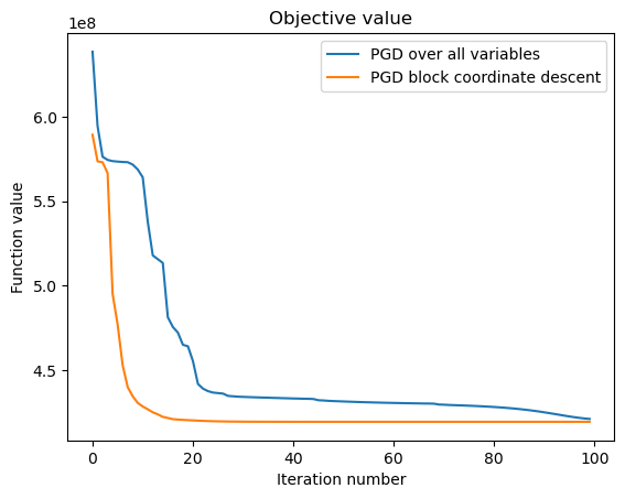
With block coordinate descent convergence is faster than optimizing all variables at the same time. This is due to the fact that each sub-problem becomes convex. Also there are some parameters that might be useful to properly tune to optimize further such as: the initialization routine, normalization steps, decreasing step size factor for backtracking, number of iterations per block, etc.

Convergence rate of the two methods implemented.

This problem has a number of particularities that could be explored in the future. For instance:

Analyzing suitable optimization routines to take advantage of the sparseness of gene expression matrices (~10% sparsity rate)
Compare different subvariants of coordinate block descent algorithms for NMF.
Incorporate known relationships between gene datasets into the problem formulation.

References

[1] “Metagenes and Molecular Pattern Discovery Using Matrix Factorization.” Accessed June 15, 2023. https://doi.org/10.1073/pnas.0308531101.

[2] “A neural network for determination of latent dimensionality in non-negative matrix factorization”

[3] Kim, Philip M., and Bruce Tidor. “Subsystem Identification Through Dimensionality Reduction of Large-Scale Gene Expression Data.” Genome Research 13, no. 7 (July 2003): 1706–18. https://doi.org/10.1101/gr.903503.

[4] Investigating the Complexity of Gene Co-expression Estimation for Single-cell Data Jiaqi Zhang, Ritambhara Singh

[5] Chapter 6 - Coordinate Descent. “Optimization for Data Analysis”. Cambridge University Press, March 2022. Stephen J. Wright and Benjamin Recht