CS826 - Theoretical Foundations of Large-Scale Machine Learning

Abstract

Inductive biases, in broad terms, guide machine learning models toward solutions with specific properties. For example, the classical inductive bias of stochastic gradient descent (SGD), studied in this class, favor minimum norm solutions. Similarly, recent developments in deep learning have introduced various definitions of inductive biases, each associated with specific assumptions and stages of the machine learning pipeline, such as the training distribution, architectural choices, and optimization algorithms. In this work, we present: 1) a comprehensive review of simplicity biases, analyzing their definitions of “simple”, underlying assumptions, and potential interrelationships. Additionaly we conduct 2) an experimental investigation quantifying these biases in multilayer perceptrons (MLPs) across different settings. Our findings reveal key dependencies between biases and provide insights into their broader implications.

A short review of modern inductive biases in deep learning (aka Simplicity biases)

Several inductive biases phenomena have been recently introduced. The following is a non-exhaustive list containing the intuition behind various forms of simplicity biases:

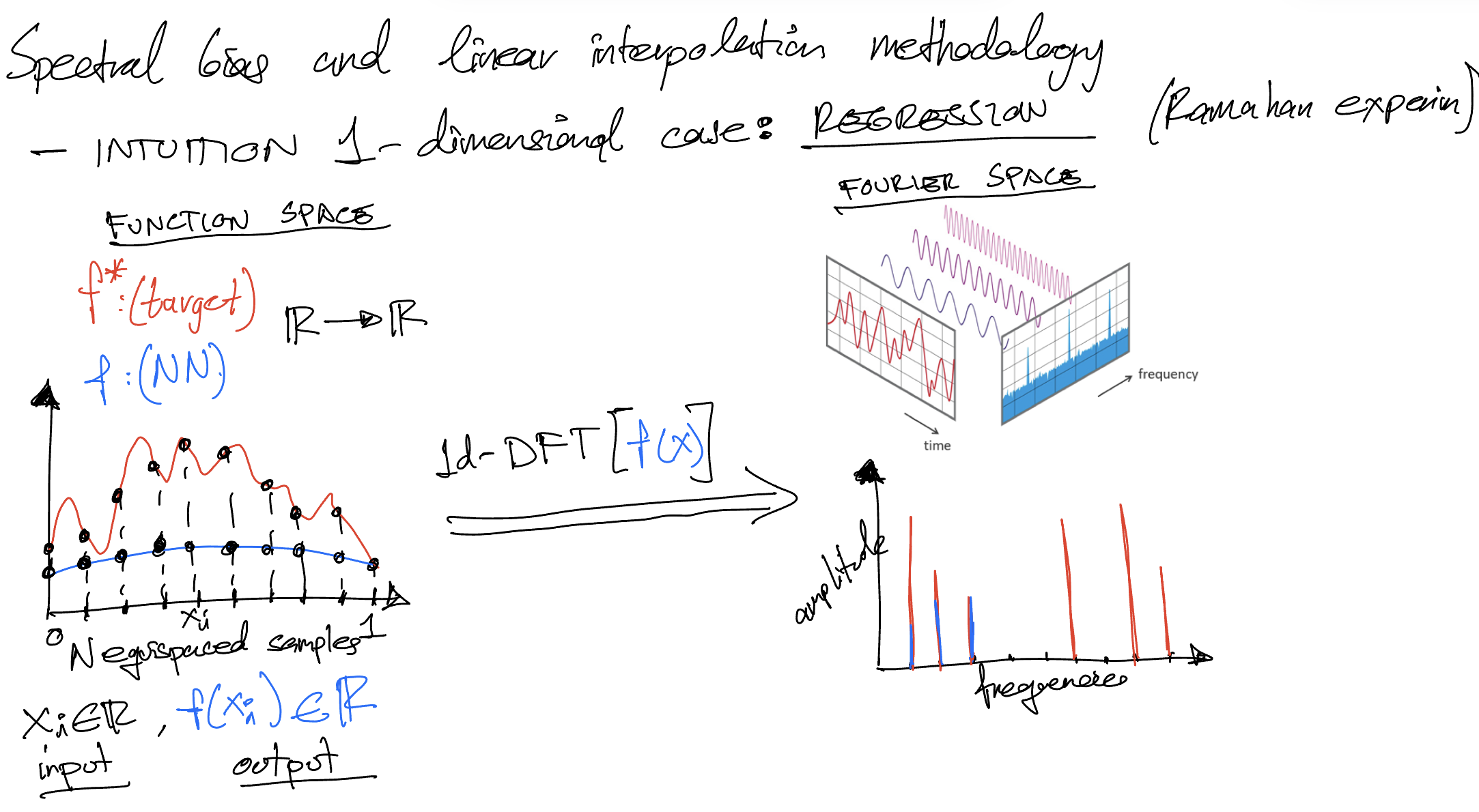
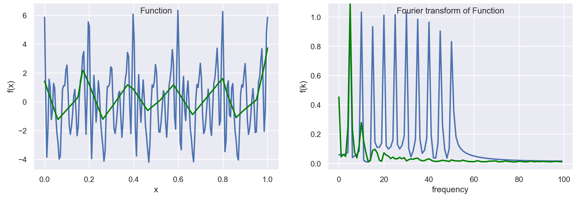
Low-frequency (Spectral) bias [1], [2], [3], [4] Deep Neural Networks (DNNs) prioritize learning low frequency functions in the Fourier space:

During training, neural networks first fit components of the target function that in the Fourier space correspond to low frequencies (functions that vary globally without local fluctuations). Higher frequencies are learned only in later epochs.
Principal component bias [5] Linear Neural Networks (LNNs) weights converge faster along the directions of principal components of data:

Linear networks parameters convergence is exponentially faster along the directions of the larger principal components of the data, at a rate governed by the corresponding singular values.
Low-dimensional input dependence bias [6], [7] DNNs output depends only on a low dimensional projection of input data:

Neural networks primarily rely on a low-dimensional subspace of the input data to label points.
Distributional bias [8], [9] DNNs learn statistics of increasing complexity:

As training progresses, neural networks exploit the lower-order statistics of the input data first (e.g. mean and covariance) before higher-order statistics (e.g. skewness and curtosis).
Low-rank (weights) bias [10] After training, Deep NN’s weights converge to rank-1 matrices
Low-rank (embedding) bias [11] DNNs learn solutions with low effective rank embeddings:

Both at initialization and after training, the feature embedding learned by the penultimate layer of neural networks have low effective rank.
Low sensitivity bias [12], [13] Transformers learn low-sensitivity functions:

During training, transformers tend to prioritize learning low-sensitivity functions—functions where the output remains relatively stable despite random perturbations in the input. This characteristic contributes to their improved robustness across a wide range of tasks.

The following comparison table summarizes their relevant properties.

Simplicity bias variant	Notion of “simple”	Assumptions on Data distribution	Assumptions on architectures	Proof that explains it	Does it hold for Strong-Performing architectures on real-world datasets?
Low-frequency (spectral)	Low frequency function (Fourier). Top Eigenfunctions of NTK (larger eigenvalues).	Uniform and Non-uniform	2-layer ReLU. Infinity-width NN	Empirical: Synthetic experiments on toy models. Theory: Spectral decomposition of NTK	CNNs on CIFAR10. ResNets, ViT and distilled Transformers on ImageNet
Principal component	Top singular vectors of covariance matrix (larger singular values) of input data	No assumptions	Overparametrized Linear NN (wide enough, any depth).	Theory: Spectral decomposition of input data covariance matrix \(XX^\top\) and analyzing \(W\) evolution in GD. line Empirical: Linear and non-linear networks.	Unknown. VGG-19 on CIFAR10
Low-dim input dependent	Low dimensional projection of the inputs.	Separable dataset. Satisfy Independent Features Model: features distributed independently conditioned on labels. Axis aligned features.	2-layer ReLU. Infinity-width NN	Theory: Kernel matrix SVM theory to NTK only considers the infty-width case. Empirical: infinity and finite-width NN on semi-synthetic datasets	Unknown
Distributional	Low order statistics of the input data	Separable on “rectangular” dataset. Axis aligned features.	Perceptron	Theory: Gradient flow of perceptron’s dynamics	DenseNet121, ResNet18 and ViT on CIFAR10
Low-rank bias (weights)	Low-rank (rank-1) weight matrices of last linear layers	Separable dataset.	Homogeneous Fully Conected ReLU NN where the last K layers are linear	Theory: Decomposition of the network	Unknown, likely no
Low-rank bias (embeddings)	Low (effective) rank of embeddings	No assumptions	Deep NN with linear and non-linear activations	Unexplored	Unknown. CNN on CIFAR/Imagenet
Low sensitivity	Low sensitivity output function wrt random changes in the input	Trransformers		Empirical: experiments on different models

Quantifying simplicity biases

Existing methodologies for measuring learning biases in SOTA networks

Methodologies for spectral bias

Previous works [1], [14] show that the learning monotonicity of DNNs stated by the spectral bias, from low to high frequencies, does not always hold. In particular, they studied spectral bias under the double descent phenomena (randomly shuffle some labels in the training set and train the network for longer epochs). [4] studied the relationship between function frequencies and input frequencies and the separation between inter-class and intra-class variance of frequency component measurements.

In low-dimensional \(x\), evaluate densely
- Sampling \(N\) evenly (equispaced) datapoints \(\{x_n\}_{n=1}^N\sim \mathcal{M}_d\) from the data manifold
- Evaluate these \(N\) points in the model. DNN outputs are \(\{f_n\}_{n=1}^N\) with \(f_n = f(x_n)\)
- Compute 1D-Discrete Fourier Transform (DFT) \(\tilde{f}_{x}(k)=\sum _{n=1}^{N}f(x_n)\cdot e^{-i2\pi {\tfrac {k}{N}}n}\)
Advantages: Easy to compute.

Disadvantage: non-tractable for large dimensional

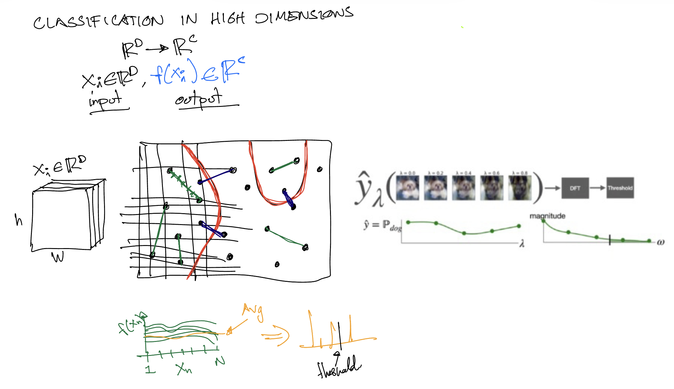
My notes on the intuition of the spectral bias in a 1-dimensional regression problem.

In high-dimensional \(x\) (e. g. image classification), perform linear interpolation [4][14]
- Randomly sample one \(\boldsymbol{\rm x} \sim \mathcal{M}_d\) (an image from the data distribution)
- Define \(f_c(\boldsymbol{\rm x})\) the \(c\)-th logit output of DNN, \(c\in \{ 1, 2, \ldots, C \}\), \(C\)= number of classes
- Interpolate linearly \(N\) points \(\{\boldsymbol{\rm x}_n\}_{n=1}^N\) (evenly) along a particular direction based on \(\boldsymbol{\rm x}\)
- Evaluate these \(N\) points in the model. DNN outputs are \(\{f_{c,n}\}_{n=1}^N\) with \(f_{c, n} = f_c(\boldsymbol{\rm x}_n)\)
- Compute 1D-Discrete Fourier Transform (DFT) \(\tilde{f}_{c, \boldsymbol{\rm x}}(k)=\sum _{n=1}^{N}f_{c}(\boldsymbol{\rm x}_n)\cdot e^{-i2\pi {\tfrac {k}{N}}n}\)
- Averaging across all dataset paths and categories \(A_k=\frac{1}{C} \sum_{c=1}^C \mathbb{E}_{x\sim D} [\tilde{f}_{c, \boldsymbol{\rm x}}(k)]^2\)
- Calculate energy ratio in log-scale: \(R_k=\log{\frac{A_k}{\sum_j A_j}}\)

My notes on the intuition of the spectral bias in a D-dimensional classification problem.

Methodologies for low-rank embedding bias

In the paper “low-rank simplicity bias in deep networks”, authors empirically observe that deeper networks are inductively biased to find solutions with lower effective rank embeddings. They particularly study the relationship between the RANK OF THE EMBEDDING and the DEPTH of neural networks. Experiments include:

Simple linear network
Over-parameterized linear network
Non-linear network

Methodologies for Principal Component bias

In the so-called “PC bias”, the convergence of weights in Deep Linear Neural Networks is governed by the eigendecomposition of raw data \(X\) when the hidden layers are wide enough. This is provably for Deep Linear NN and empirically for Nonlinear NN. PC bias is introduced as a generalization (extension from single-layer to deep) of the known behavior of the single-layer convex linear model. The authors also relate PC bias phenomena with early stopping and slower convergence rate with shuffle labels.

Assumptions: LNN optimized with GD. No assumptions on dataset separability.
Weight evolution: They derive the temporal dynamics of compact representation \(W\) as it changes with each GD step. Gradient descent guides the network to first learn the features that carry more information from data (have higher singular value)!

PC-bias implementation:

Train DLNN on rotated data \(\boldsymbol{U^TX}\)
Compute their compact representation \(\boldsymbol W^* = \prod_{l=L}^1 W_l^*\)
Two options:
- Do inference with \(\boldsymbol W^*\) using rotated test data \(\boldsymbol{U^TX}\)
- Do inference with unrotated weights \(\boldsymbol{W^*U^T}\) using original test data \(X\)

To measure PC-bias across iterations we need:

Compact representation \(W\) of the network (closest to nonlinear model)
Measure convergence along each dimension separately
- Train \(N\) models independently
- Compute its compact representation \(W\)
- Compute the standard deviation of \(W\) per dimension

Experiments and preliminary results

Many of the previous bias definitions were originally validated in simple theoretical scenarios only, e.g. single or two-layer neural networks, linear networks, etc. Thus, their consistency across a variety of configurations is not clear. In this work we perform experimentation to answer questions of the type:

To what extent each bias depends on data, architecture and optimizer?

We aim to measure to what extend each biasing mechanism depends on the data, architecture or optimizer. For instance we want to verify if the bias in wide (and shallow) networks is the same from the biasing mechanism in deep (and narrow) networks. Similarly, we would like to evaluate their interplay across:

Dataset: Randomly (uniformly), Non-uniform, Different data distribuition.
Architecture: Activations (ReLu, Tanh, Linear), Overparametrization (Depth, Width)
Optimization: Weight initialization, SGD, AdamW

Spectral bias dynamics measured in a 10-layer deep, 256-wide MLP. Top left: target function (blue) and function predicted at first epoch (green). Top right: Fourier transform of target function (blue) and Fourier transform of predicted function (green). Bottom left: Frequencies learned across iterations. Bottom right: Training curve.

After the experimentation described, firstly we summary the stages where each phenomenon is observed:

When each bias phenomenon is observed?

Secondly, it is worth noticing the different spaces that are interacting when these biases occur:

Input space (\(\mathcal{D}\)-space): Characterizes the features of the training data distribution that influence the network.
Parameter space (\(\theta\)-space): Parametrize the function space chosen.
Hypothesis/Function space (\(\mathcal{H}\)-space): Characterize the function that the network learns.
Fourier space (\(\mathcal{F}\)-space): Frequency domain of the function

CS826 - Theoretical Foundations of Large-Scale Machine Learning

Quantifying modern inductive biases for deep learning

References

- On the Spectral Bias of Neural Networks, Rahaman et. al. ICML 2019
- Towards Understanding the Spectral Bias of Deep Learning, Cao et. al. IJCAI 2021
- Frequency Bias in Neural Networks for Input of Non-Uniform Density, Basri et. al. ICML 2020
- Spectral Bias in Practice: the Role of Function Frequency in Generalization, Fridovich-Keil et. al. NeurIPS 2022
- Principal Components Bias in Over-parameterized Linear Models, and its Manifestation in Deep Neural Networks, Hacohen et. al. JMLR 2022
- The Pitfalls of Simplicity Bias in Neural Networks, Shah et. al. NeurIPS 2020
- Simplicity Bias in 1-Hidden Layer Neural Networks, Morwani et. al. NeurIPS 2023
- Neural Networks Learn Statistics of Increasing Complexity, Belrose et. al. ICML 2024
- Neural networks trained with SGD learn distributions of increasing complexity, Refinetti et. al. ICML 2023
- Training invariances and the low-rank phenomenon: beyond linear networks, Le et. al. ICLR 2022
- The Low-Rank Simplicity Bias in Deep Networks, Huh et. al. TMLR 2023
- Simplicity Bias in Transformers and their Ability to Learn Sparse Boolean Functions, Bhattamishra et. al. ACL 2023
- Simplicity Bias of Transformers to Learn Low Sensitivity Functions, Vasudeva et. al. ArXiv 2024
- Rethink the Connections among Generalization, Memorization, and the Spectral Bias of DNNs, Zhang et. al. IJCAI 2021