CS 838 Pervasive Parallelism Fall 2005 Section 3 Instructor Mark D. Hill URL: http://www.cs.wisc.edu/~markhill/cs838/Fall2005/

Homework 2 // Due at Lecture Wednesday, September 21, 2005

Please direct questions to Michelle Moravan (moravan@cs...) who helped create this assignment.

Perform this assignment on cabernet.cs.wisc.edu, a 16-processor Sun E6000, where we have activated a CS account for you. (Unless you already had an account, you should only use this machine only for 838-3 homework assignments or your course project. Unless you have a longer connection for CS, this account and its storage will be removed after the end of the semester.)

You should do this assignment alone. No late assignments.

Purpose

The purpose of this assignment is to give you experience writing a shared memory program with pthreads to build your understanding of shared memory programming, in general, and pthreads, in particular.

Programming Environment: Pthreads

The methods of communication and synchronization are two characteristics that define a parallel programming model. In your MPI program, you explicitly specified communication by passing messages between processors. Synchronization occurred implicitly as processors used the information in these messages to update their local states.

A threaded model reverses these properties. While in MPI each processor had its own, private address space, with threads, all processors access a single address space (hence the name "shared memory"). Thus, communication occurs implicitly, because whenever one thread writes to an address, the update is immediately visible to all others. On the other hand, this introduces the need for explicit synchronization to avoid races among multiple processors to access data at the same address.

Different systems support threads in a variety of ways. For this assignment, you will use Posix Threads, or pthreads for short. One advantage of this particular implementation is its portability to many different systems. Do man pthreads from cabernet to see a summary of pthreads functions. You can find details for any listed function by doing man function_name. Note that the man page also includes information about Solaris threads. For this assignment, you should use Posix threads, not Solaris threads.

All threaded programs begin with a single thread. When you reach a section you wish to do in parallel, you will "fork" one or more threads to share the work, telling each thread in which function to begin execution. Keep in mind that the original, "main" thread continues to execute the code following the fork. Thus, the thread model also provides "join" functionality, which lets you tell the main thread to first wait for a child to complete, and then merge with it.

It is likely that you will have many threads execute the same routine, and that you will want each thread to have its own private set of local variables. With pthreads, this occurs automatically. Only global variables are truly shared.

When you have multiple threads working on the same data, you may require synchronization for correctness. Pthreads directly supports two techniques: mutual exclusion (locks) and condition variables. A third technique you may find useful is barriers. A barrier makes all threads wait for each other to arrive at a certain point in the code before any of them can continue. While pthreads offers no direct barrier support, you should be able to build a barrier of your own out of the mutual exclusion primitive.

A final issue with threads is how they are mapped to processors. Obviously, we can have more threads than processors, but someone must then time multiplex the threads onto the processors. Since this is probably more complexity than you want to deal with, we recommend that you directly bind each thread to a particular processor. More precisely, on Solaris we actually bind threads to light-weight processes (LWP's), but all you really need to know is that by binding threads, you transfer responsibility for contention management of threads on processors to the operating system.

In order to use pthreads on cabernet, you must compile with cc (not GCC or G++). Any source files that call pthread library functions must include the pthread.h header file. Additionally, the flags -mt -lpthread must be passed to cc for both compilation and linking.

For more information:

• The pthreads example program demonstrated in class is available for review here: tar.gz or zip.
• This tutorial from Lawrence Livermore is also an excellent reference.

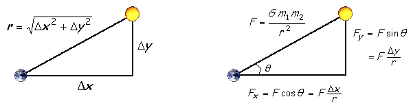
Programming Task: N-Body Simulation

An n-body simulation calculates the gravitational effects of the masses of n bodies on each others' positions and velocities. The final values are generated by incrementally updating the bodies over many small time-steps. This involves calculating the pairwise force exerted on each particle by all other particles, an O(n²) operation. For simplicity, we will model the bodies in a two-dimensional space.

The physics. We review the equations governing the motion of the particles according to Newton's laws of motion and gravitation. Don't worry if your physics is a bit rusty; all of the necessary formulas are included below. We already know each particle's position (r_x, r_y) and velocity (v_x, v_y). To model the dynamics of the system, we must determine the net force exerted on each particle.

• Pairwise force. Newton's law of universal gravitation asserts that the strength of the gravitational force between two particles is given by the product of their masses divided by the square of the distance between them, scaled by the gravitational constant G, which is 6.67 × 10^-11 N m² / kg². The pull of one particle towards another acts on the line between them. Since we will be using Cartesian coordinates to represent the position of a particle, it is convenient to break up the force into its x and y components (F_x, F_y) as illustrated below.
  
• Net force. The principle of superposition says that the net force acting on a particle in the x or y direction is the sum of the pairwise forces acting on the particle in that direction.

• Acceleration. Newton's second law of motion postulates that the accelerations in the x and y directions are given by: a_x = F_x / m, a_y = F_y / m.

The numerics.  We use the leapfrog finite difference approximation scheme to numerically integrate the above equations: this is the basis for most astrophysical simulations of gravitational systems. In the leapfrog scheme, we discretize time, and update the time variable t in increments of the time quantum Δt. We maintain the position and velocity of each particle, but they are half a time step out of phase (which explains the name leapfrog). The steps below illustrate how to evolve the positions and velocities of the particles.

For each particle:

1. Calculate the net force acting on it at time t using Newton's law of gravitation and the principle of superposition.

2. Calculate its acceleration (a_x, a_y) at time t using its force at time t and Newton's second law of motion.

3. Calculate its velocity at time t + Δt / 2 by using its acceleration at time t and its velocity (v_x, v_y) at time t - Δt / 2. Assume that the acceleration remains constant in this interval, so that the updated velocity is:   v_x = v_x + Δt a_x,   v_y = v_y + Δt a_y.

4. Calculate its position at time t + Δt by using its velocity at time t + Δt / 2 and its position at time t. Assume that the velocity remains constant in the interval from t to t + Δt, so that the resulting position is given by r_x = r_x + Δt v_x,   r_y = r_y + Δt v_y. Note that because of the leapfrog scheme, the constant velocity we are using is the one estimated at the middle of the interval rather than either of the endpoints.

As you would expect, the simulation is more accurate when Δt is very small, but this comes at the price of more computation.

Problem 1: Write Sequential N-Body

Write a single-threaded solution to the n-body problem described above. Your program should take as input the number of particles, the length of the time-step Δt, and the number of these time-steps to execute. Your final version should randomly generate the mass, x and y Cartesian coordinates, and x and y velocity components for each particle, then simulate for the specified number of time-steps.

For the randomly generated values, you may use any range that you like. However, if you have very large masses which happen to be initialized to positions that are very close to each other, you may encounter overflow. Since the focus of this assignment is parallel programming and scalability, you will not be graded on elegantly handling or avoiding such situations.

You are required to make an argument that your n-body implementation is correct. A good way to do this is to initialize the bodies to a special-case starting condition, and then show that after a number of time steps the state of the grid exhibits symmetry or some other expected property. You need not prove your implementation's correctness in the literal since. However, please annotate any simulation outputs clearly.

Problem 2: Write Pthreads N-Body

For this problem, you will use pthreads to parallelize your program from Problem 1. This program should take an additional command-line argument: the number of threads to use in the parallel section.

It is only required that you parallelize the main portion of the simulation, but parallelizing the data generation phase of your n-body program is also worthwhile. You will not be penalized if you choose not to parallelize the initialization phase.

To ensure that you have some practice with mutual exclusion, your parallel n-body program must use at least one lock. One way to satisfy this requirement is to implement your own barrier.

For simplicity, you may assume that the number of bodies is evenly divisible by the number of threads.

Problem 3: Analysis of N-Body

In this section, you will analyze the performance of your two N-Body implementations.

Modify your programs to measure the execution time of the parallel phase of execution. If you chose to parallelize the data generation phase, you may include that as well. Either way, make it clear exactly what you are measuring. Use of Unix's gethrtime() is recommended. Do not use the built-in TCL time command.

Plot the normalized (versus the serial version of n-body) speedups of Program 2 on N=[1,2,4,8,16] for 512 bodies and 1000 time steps. The value of dt is irrelevant to studying scalability: with the number of time steps held constant, it only affects the length of time simulated, not the duration of the simulation itself. Thus you may choose any value you like. We recommend that you use multiple trials in conjunction with some averaging strategy. Describe the procedure you used.

Tips and Tricks

• Start early.
• Make use of the demo programs provided.
• You can use /usr/platform/sun4u/sbin/prtdiag -v on cabernet to learn many useful characteristics of your host machine.
• When scrutinizing your program for correctness, remember that too large a time-step can dramatically affect your results.
• The unique identifiers returned by pthread_self() do not necessarily range from 0 to the total number of threads.
• If you parallelize the data generation phase and compare the results to your sequential program, even using the same random seed, why might the results differ?

What to Hand In

Please turn this homework in on paper at the beginning of lecture. You must include:

• A printout of the simulation phase of Program 1.
• A printout of the parallel phase of Program 2.
• Arguments for the correctness of Programs 1 and 2.
• The plot as described in Problem 3, including labels describing your data.

Important: Include your name on EVERY page.