Causal inference can prevent computer vision from falling into black-box deep learning
- Homework 1
- Homework 2
- Homework 3
- Homework 4
-
Homework 5
- What assumptions have I made that are important to my inferences/conclusions?
- What alternatives to estimation/implementation/identification are available to investigate the sensitivity of my conclusions/inferences to my assumptions?
- How would your inferences/conclusions change (if at all) if your assumptions were violated?
- What assumptions (if at all) cannot be investigated in any principled way?
- Homework 6
- References
Homework 1
Who am I?
My name is Mu Cai. Currently, I am a third-year Ph.D. student in the Department of Computer Sciences at the University of Wisconsin- Madison, supervised by Prof. Yong Jae Lee. I got my bachelor’s degree in Electrical Engineering and Automation at Xi’an Jiaotong University in 2020. My research interest lies in the intersection of deep learning and computer vision. I am especially interested in 3D scene understanding and self-supervised learning. You can find more information here.

What are my professional preparation/interests, background, and goals?
I am a Ph.D. student with a computer science background. I am also interested in mathematics-driven data science, where math (will) become my minor. Most of the time, I use deep learning, the well-known black box but powerful tool, to empirically improve the performance of computer vision problems. I am passionate about solving real world problems that better serve people, such as 3D perception in autonomous driving. However, current deep learning-based approaches may not reveal the underline relationship between objects and labels. For example, recent studies found that the irrelevant background could be an informative feature when recognizing the foreground objects, known as supurious correlation. A straightforward idea is: can we use the well-established causal inference to help improve the reliability of deep learning?
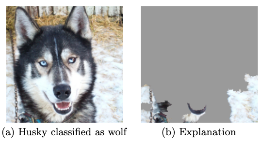
Why am I interested in causal inference?
Therefore, the causal inference may provide us with a way to build an interpretable computer vision framework. Other areas, such as vision-question-answering (VQA), can also be equipped with causal inference to improve both final performance and interpretation.
Homework 2
What question do you want to answer? And why is it important to answer it?
Deep learning has achieved great success in a wide spread of pattern recognition problems, including computer vision [Ren et al. 2015], natural language understanding, and reinforcement. However, deep neural networks have been criticized as a “function approximator”, i.e., it doesn’t learn the true “intelligence”. Instead, neural networks could just be a mapping from the feature to the label for the majority of samples. Therefore, the under-represented groups may be incorrectly predicted in a biased way. For example, here we consider a computer vision task called scene graph generation. We are given the objects and their bounding boxes.
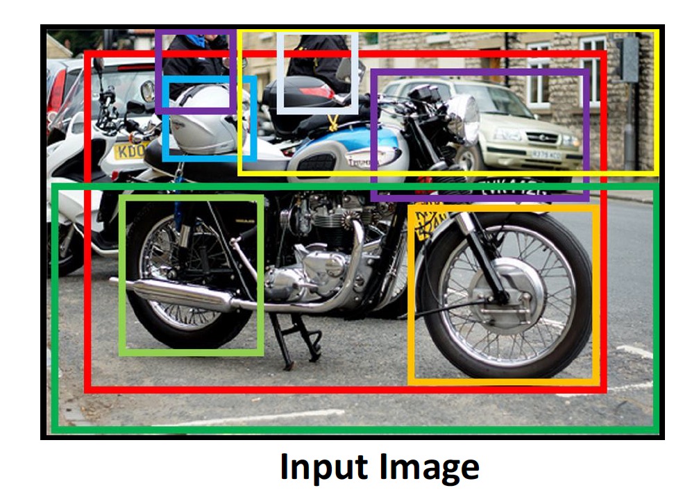
We are supposed to generate a scene graph [Tang et al. 2020] that describes the relationship between the objects, as the right figure shows in the below image. However, actually, we can only get the (left) biased scene graph where the descriptions are vague and don’t represent the accurate action or location information. For example, in the biased generations, there are a lot of words like “on, has, near”, instead of the the correct descriptions like “behind, parked on”.

Why could this happen? The major reason is that for the ease of annotation, most of the text descriptions in the training set are composed of common words like “has, on, wearing”. Therefore, neural networks just learn such common words, and may not reflect the underrepresented actions/relationships. Therefore, it is important to correctly represent the scene graph using a proper inference scheme.
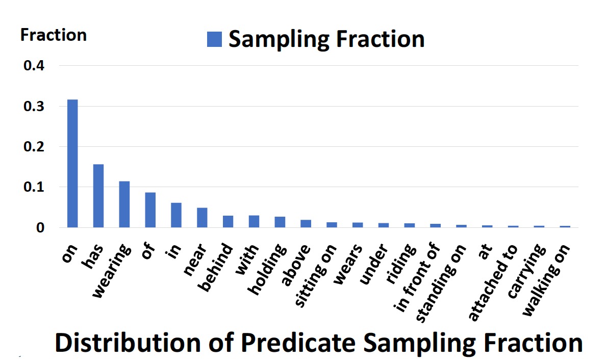
Causal inference can be a great fit for this problem. Given the objects, how can we find the proper relationship between them? We may use the intervention model or the counterfactual causality to tackle this problem. We can also expand our analysis to other vision tasks like Vision-Question-Answer (VQA) [Wang et al. 2020]. I also plan to integrate language features into the framework to improve the final performance on tasks like scene graph generation. This approach can also improve the robustness of the interpretation ability of neural networks.
What (observed or unobserved) random variables are needed to fully model the problem?
Here we need 4 random variables to fully model our problem. They are all observed variables under the current problem setting. Here \(I\) denotes the image, which can be represented as the high-level semantic features from a feature extractor backbone. \(X\) denotes the object features, which are also the feature maps in the deep neural network. \(Z\) denotes the object labels. \(Y\) denotes the predicated logits.
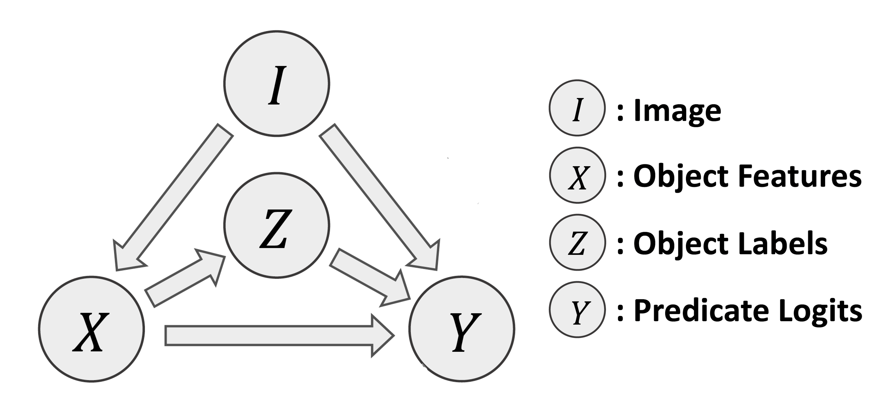
Here is a concrete example, where the nodes and links in DAG are clearly presented.
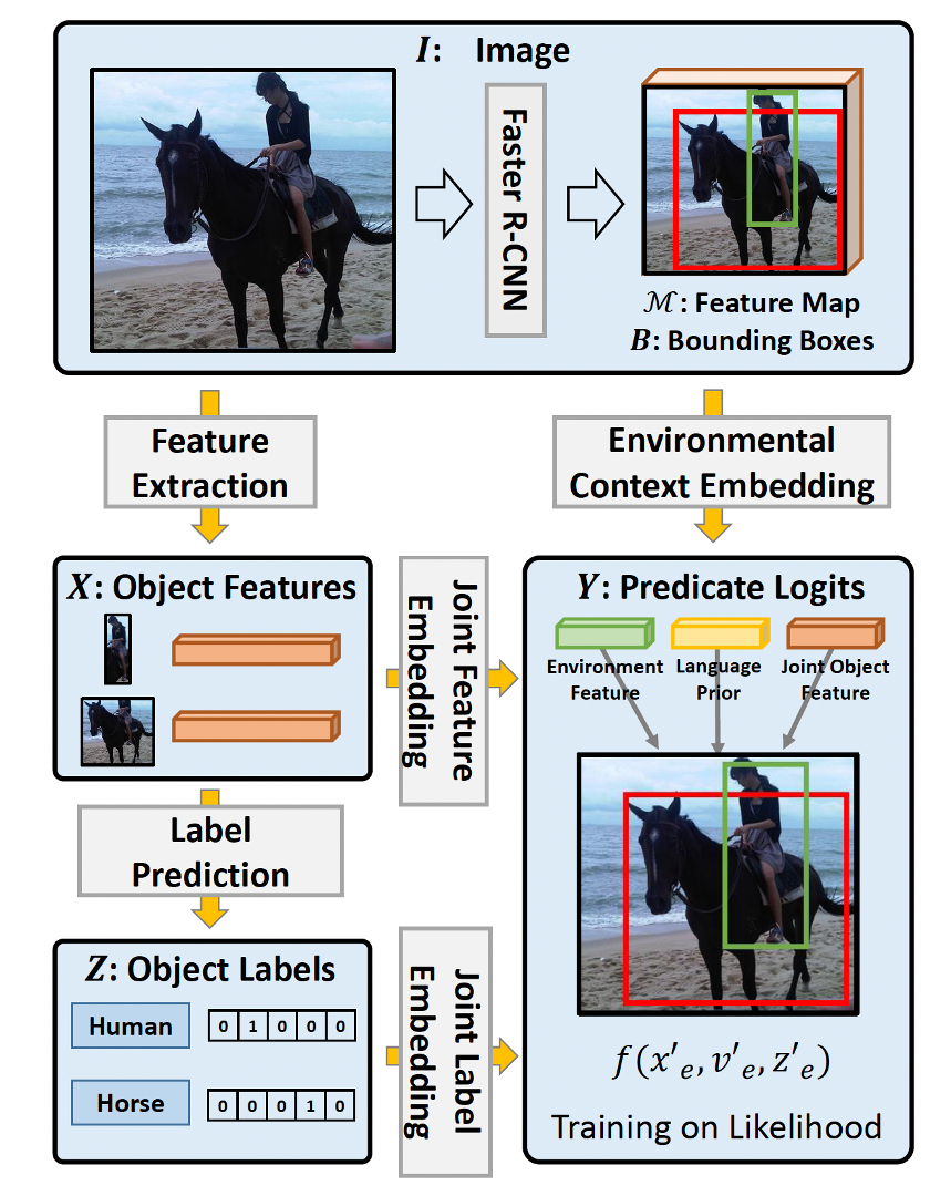
What is the causal effect that you wish to study?
Here I want to study the Total Direct Effect [VanderWeele et al. 2020] [Tang et al. 2020].
\[T D E=Y_x(i)-Y_{\bar{x}, z}(i),\]where \(Y_x(i)\) is the observed outcome. Here I would like to use counterfactual causality based on the intervention \(X=\bar{x}\) to conduct the analysis. Thus the first term is from the original graph and the second one is from the counterfactual. Within this process, do-calculus is also introduced, e.g., \(do(X=\bar{x})\).
What are your working hypotheses about the relationship between variables?
Here I am also working with DAG. From my problem setting, we know that all edges are directed, and there are no cycles. Therefore, we can say that it has a topological or causal ordering. Three assumptions in the potential outcome framework can also be applied here.
Homework 3
Assumptions made for identification, and reasons
I will still use the causal graph depicted in Homework 2.
Here we need 4 random variables to fully model our problem. They are all observed variables under the problem setting. Here \(I\) denotes the image, which can be represented as the high-level semantic features from a feature extractor backbone (which can be viewed as confounder). \(X\) denotes the object features, which also feature maps in the deep neural network (can be viewed as the treatment). \(Z\) denotes the object labels. \(Y\) denotes the predicated logits for object relationships (can be viewed as the treatment effect).

As my previous causal graph shows, my graph is a directed acyclic graph (DAG), which satisfies two properties in its definition: (1) All edges are directed, and (2) There are no cycles.
Here it satisfied three assumptions: consistency, SUTVA, and exchangeability. The explanations are:
(a) Consistency. The potential outcome if we were to assign intervention \(X\) (object features) is exactly \(Y\) (object relationships in the scene), i.e. \(Y=Y(X)\).
(b) SUTVA (stable-unit value assumption). The mapping \(x \mapsto Y(x)\) is a well-defined function from \({X}\) to the set of random variables (i.e. real-valued measurable functions) defined on our probability space. Here \(x\) is object features.
(c) Exchangeability. Potential outcomes (object relationships) \(Y(x)\) are independent from the treatment assignment (here is object features) \(X\) for each \(x \in {X}\).
\[Y(x) \perp X, \quad x \in X\]In our causal grapth, we also need to condition on \(I\) to let \(Y(x) \perp X\).
Besides, the positivity (common support) can not be viewed as valid. This is because the object features are extracted from an image feature extractor. Therefore, to do identification, I use the method of counter-factual to build such “pseudo” positivity.
According to my explanation and the DAG visualization, the assumptions and claims are valid.
Steps needed for identification and Justification for each step
Here I will use do calculus to build my intervention mode, which is used in the single world intervention graphs.
\[do(X=\bar{x})\]Here my intervention action denotes whether I use the original object features \({x}\) or whether I use the counterfactual object features \(\bar{x}\), which is described in detail in the next subsection.
After using the counterfactual object features \(\bar{x}\), which are the mean feature values across the dataset, we can get a graph like this
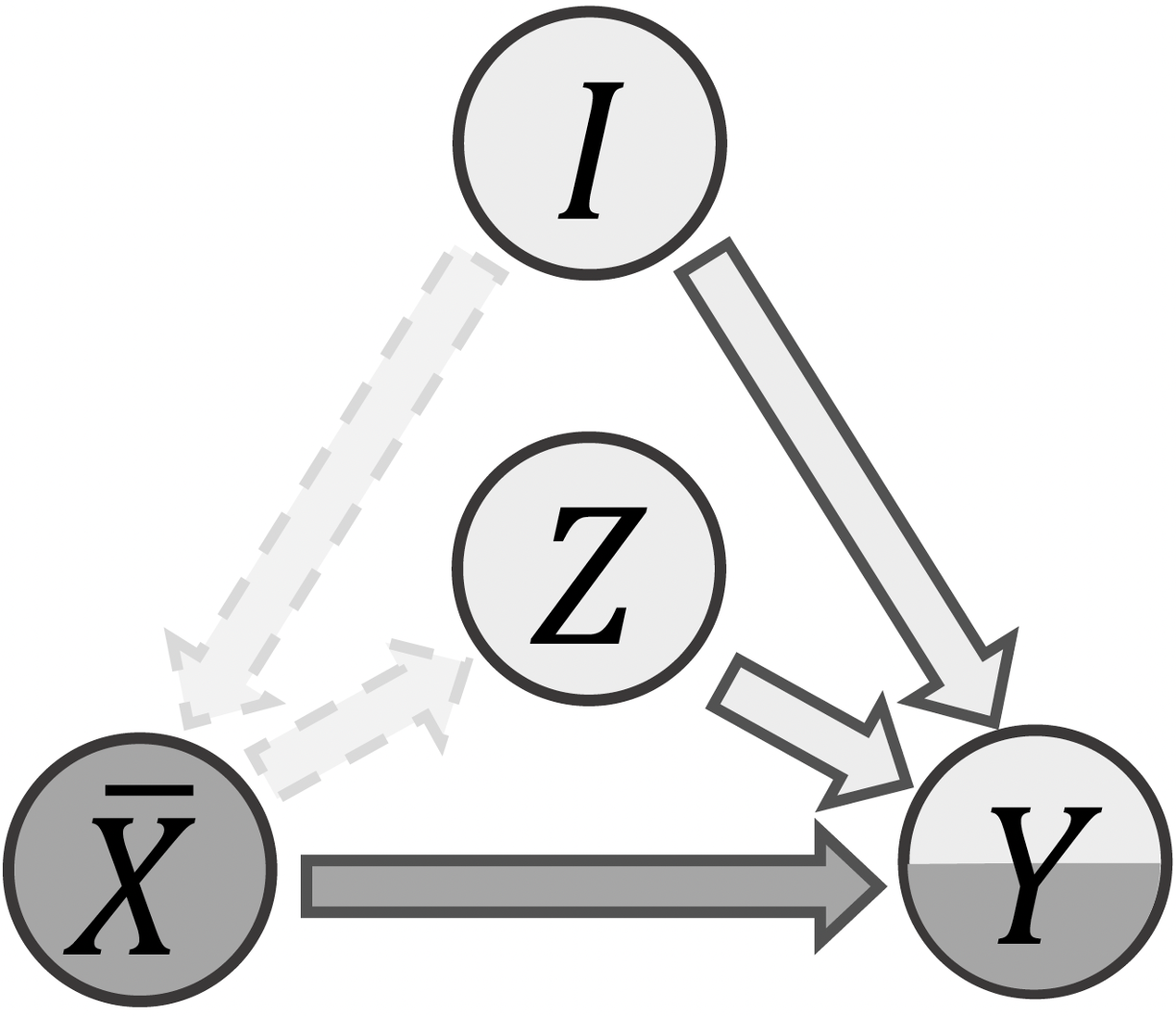
We can see the two dashed lines are removed from the original graph. This is because of the basic components in the graph, using d-separation. \(X \rightarrow Z\) is a pair in a chain \(X \rightarrow Z \rightarrow Y\) starting from \(X\), and \(X \leftarrow I\) is a pair in a chain in a collider \(X \leftarrow I \rightarrow Y\) . When conditioned on (controlling) the \(X\), then the following three casual relationships would be eliminated:
(1) \(X \rightarrow Z\): \(X\) and \(Z\) would be independent given \(x\).
(2) \(I \rightarrow X\). \(X\) and \(I\) would be independent given \(x\).
(3) \(X \rightarrow Y\). \(X\) and \(Y\) would be independent given \(x\).
We need to identify \(E[Y(x, i, z \mid X=x))]\). The analysis can be done using a similar analysis in g-formula.
Use Markov compatibility to get \(Y(x, i, z \mid X=x) \perp X\), and
\[E[Y(x, i, z \mid X=x))] = E[Y(x, i, z)]\]Use Markov compatibility to get \(Y(x, i, z) \perp X, I, Z\), and
\[E[Y(x, i, z)] = E[Y(x, i, z) \mid X=x, I=i, Z=z]\]Using consistency, we get
\[E[Y(x, i, z) \mid X=x, I=i, Z=z] = E[Y \mid X=x, I=i, Z=z]\]Interpretation for the conclusions from the identification proof
In class, we talk about the concept the ADE (average treatment effect). However, we have a “fixed” variable for the object feature, and we want to study the effect of each object feature for the corresponding image itself, not across the whole dataset. Since every feature of the image is unique, then we can replace \(E[Y \mid X=x, I=i, Z=z]\) with \(Y(x, i, z)\). Therefore, we can use the method called counterfactual causality, which can replace \(X\) with the zeros values or the mean feature values across the dataset, called \(\bar{x}\). Here we fix the value for the parents of \(x\) [VanderWeele et al. 2020], i.e., the overall image feature \(i \in I\) and the object labels. Thus we get \(Y(\bar{x}, i, z)\). There we can use the difference value of the original inference result \(Y(x, i, z)\) and the counterfactual inference results \(Y(\bar{x}, i, z)\) to show such a gap for the outcome \(Y\). Here \(Y\) follows a distribution for a discrete set, thus we can represent the true object relationship using \(y \in Y\) with the largest gap.
To be more specific, total direct effect [VanderWeele et al. 2020] is:
\[T D E=Y(x, i, z)-Y(\bar{x}, i, z),\]where \(Y(x, i, z)\) is the observed outcome.
Then we can see how \(Y\) would change under original object features \(x\) and the counterfactual features \(\bar{x}\). For example, \(Y\) could be sampled from a set of object relationships such as “on”, “near”, and “sitting on”. Then the resulting estimated object relationship would be the \(Y\) with maximum total direct effect(TDE).
Homework 4
What algorithms are used for estimation/implementation?
I use a similar approach to matching, which is counterfactural anaylsis. To be specific, I adopt the method of exact matching. Similar to what I did in Homework 3, I re-emphasize the assumptions I made for identification.
As my previous causal graph shows, my graph is a directed acyclic graph (DAG), which satisfies two properties in its definition: (1) All edges are directed, and (2) There are no cycles.
Here it satisfied three assumptions: consistency, SUTVA, and exchangeability. The explanations are:
(a) Consistency. The potential outcome if we were to assign intervention \(X\) (object features) is exactly \(Y\) (object relationships in the scene), i.e. \(Y=Y(X)\).
(b) SUTVA (stable-unit value assumption). The mapping \(x \mapsto Y(x)\) is a well-defined function from \({X}\) to the set of random variables (i.e. real-valued measurable functions) defined on our probability space. Here \(x\) is object features.
(c) Exchangeability. Potential outcomes (object relationships) \(Y(x)\) are independent from the treatment assignment (here is object features) \(X\) for each \(x \in {X}\).
\[Y(x) \perp X, \quad x \in X\]In our causal grapth, we also need to condition on \(I\) to let \(Y(x) \perp X\).
What steps are needed for estimation/implementation?
As methioned in Homework3, I use Total Direct Effect [VanderWeele et al. 2020] [Tang et al. 2020] to characterize the casual effect.
In class, we talk about the concept the ADE (average treatment effect). However, we have a “fixed” variable for the object feature, and we want to study the effect of each object feature for the corresponding image itself, not across the whole dataset. Since every feature of the image is unique, then we can replace \(E[Y \mid X=x, I=i, Z=z]\) with \(Y(x, i, z)\). Therefore, we can use the method called counterfactual causality, which can replace \(X\) with the zeros values or the mean feature values across the dataset, called \(\bar{x}\). Here we fix the value for the parents of \(x\) [VanderWeele et al. 2020], i.e., the overall image feature \(i \in I\) and the object labels. Thus we get \(Y(\bar{x}, i, z)\). There we can use the difference value of the original inference result \(Y(x, i, z)\) and the counterfactual inference results \(Y(\bar{x}, i, z)\) to show such a gap for the outcome \(Y\). Here \(Y\) follows a distribution for a discrete set, thus we can represent the true object relationship using \(y \in Y\) with the largest gap.
To be more specific, total direct effect [VanderWeele et al. 2020] is:
\[T D E=Y(x, i, z)-Y(\bar{x}, i, z),\]where \(Y(x, i, z)\) is the observed outcome.
Then we can see how \(Y\) would change under original object features \(x\) and the counterfactual features \(\bar{x}\). For example, \(Y\) could be sampled from a set of object relationships such as “on”, “near”, and “sitting on”. Then the resulting estimated object relationship would be the \(Y\) with maximum total direct effect(TDE).
The concrete steps (pseudo-code) of algorithm:
def causal_inference_scene_graph(neural_network, raw_image, threshold = 0.2, training= False, loss_fn = CrossEntropy, gt_relationship = None, use_TDE=True):
    """ casuality estimation using total direct effect

    Parameters
    ----------
    neural_network : convolution neural network trained by the object detection
    objective.
    raw_image : tensor with shape [3, H, W]
        Here 3 is the number of channles for the image, which is RGB,
        H and W are the height and width of the image.
    threshold: threshold value for the casaulity value.
    training: whether the model is in the training or validation stage.
    gt_relationship: the ground truth human annotated object relationship (casual relationship) in the training stage.
    use_TDE: whether we use use_TDE or not

    Warnings
    --------
    This function can be utilized in both training and inference.

    Returns
    -------
    causal_list : casuality estimation list with  shape [N, 2],

    """

    # Get the image feature I and the bounding boxes prerdicted by the neural network
    # I is the tensor with shape [C, H', W']
    # boundingboxes has the shape of [N, 4], where N is the number of
    I, boundingboxes, Y, Z = neural_network.backbone(raw_image)
    # Get the object features by cropping the overall image features I using boundingboxes
    X = FeatureExtraction(I, boundingboxes)
    # Get object labels usingg label_prediction from the neural network
    Z = neural_network.label_prediction(X)

    if use_TDE:
        # get the counterfactual object feature representation by taking the average of all object features
        mean_feature_value = torch.mean(X, dim =0 )
        x_bar = mean_feature_value

    causal_list = []

    # we can detect many pairs of object,
    for x1,z1 in zip(X, Z):
        for x2,z2 in zip(X, Z):
            # concate two objects features x and their corrsponding labels z
            x = torch.cat([x1, x2])
            z = torch.cat([z1, z2])
            # predict the effect using treatment, which is a vector in R^K, where K is the number of possible
            Y = neural_network.object_relationship_prediction(I, x, z)
            # if we are in the training stage, conduct gradient decent for the object_relationship_prediction branch.
            if training:
                loss = loss_fn(gt_relationship, Y)
                loss.backward()
            if use_TDE:
                # predict the counterfactual effect
                Y_bar = neural_network.object_relationship_prediction(I, xbar, z)
                # get total direct effect
                TDE=Y-Y_bar
                # if TDE is larger than a manually decided threshold, then add it to the output lits
                if TDE>threshold:
                    causal_list.append([z, TDE.argmax()])
            else:
                # use the normal object relationship using argmax
                causal_list.append([z, Y.argmax()])

    # return the final causal relationship list
    return causal_list
How exactly does data factor into estimation/implementation?
I use the realworld 2D images with common objects to conduct causal reasoning. Specifically, I use the Visual Genome (VG) [Krishna et al. 2017] dataset. The dataset is composed of 108k images across 75k object categories and 37k predicate relationship. We split the overall dataset into the training set (70%) and test set (30%).
As I mentioned in the previous section, during the inference stage, the input is just the raw image with \(I \in \mathbb{R}^{3\times H \times W}\), where \(H\) and \(W\) denotes the height and width of the image, respectively.
However, before the inference stage, we need a well trained model that can detect the objects and their
associated bounding boxes well. Nowadays, researcher mainly adopt neural networks, in particular,
convolution neural networks [He et al. 2017] or transformers[Carion et al. 2020], to conduct 2D object detection. During such training stage,
we feed the \(I \in \mathbb{R}^{3\times H \times W}\) and the bounding boxes annotations \(B \in \mathbb{R}^{N \times 4}\), where \(N\) is the number of boxes, \(B_i\) denotes the upperleft and lower right coordinates for the specific box \(i\). In our context, neural_network.backbone would serve as the module to extract the bounding boxes. Here we use a pretrained Mask-RCNN [He et al. 2017] model.
Besides, if we directly inference the object relationships using counterfacial resoning, the result would not be promising.
Since scene graph generation problem aims at investigating the casual relationship for each image, we can annotate a bunch of
training samples, and use evaluate the performance under the test set. Therefore, we would also provide the causal relationship ground truth \(C \in \mathbb{R}^{M}\), here \(M\) denotes the number of casual relationships annotated by human. After training stage, neural_network.object_relationship_prediction would be ready to use for object relationship prediction, whether by normal softmax prediction or via causal inference (TDE).
The results/performance of the algorithm?
The results coorespond to our expectation. We evaluete the performance under the standard metrics in scene graph generation (SGG).
For the theoretical or practical properties of the algorithm, since we are coundcting causal inference on the single image, the consistency would be naturally satisfied. Bias would be a major consideration here. Since human annotators tend to use simple relationship to annotate the dataset, which could save their time, thus the vanilia causal inference results would highly lean towards the most frequency object relationship catogories. The algorithm would be efficient, due to the nature of the feed-forward neural network.
Firstly, we show the results for an example image. For each detected bounding box, the index and the catogory are shown on the upperleft corner of the box.

Here we show the top 20 object relationships discovered by the normal argmax operation and our total direct effect casuality estimation.
** Normal (Vanilia) argmax estimation **

**************************************************
rel_labels 0: 1_man => wearing => 7_jacket; score: 0.48118364810943604
rel_labels 1: 6_man => wearing => 5_pant; score: 0.46438875794410706
rel_labels 2: 1_man => wearing => 11_pant; score: 0.42527636885643005
rel_labels 3: 6_man => wearing => 8_shirt; score: 0.39771541953086853
rel_labels 4: 6_man => wearing => 3_jacket; score: 0.3942137360572815
rel_labels 5: 6_man => on => 9_sidewalk; score: 0.018205227330327034
rel_labels 6: 1_man => on => 9_sidewalk; score: 0.013966969214379787
rel_labels 7: 2_tree => on => 9_sidewalk; score: 0.008086176589131355
rel_labels 8: 5_pant => on => 6_man; score: 0.0014106290182098746
rel_labels 9: 11_pant => on => 1_man; score: 0.0011337836040183902
rel_labels 10: 8_shirt => on => 6_man; score: 0.0011065977159887552
rel_labels 11: 3_jacket => on => 6_man; score: 0.000999525422230363
rel_labels 12: 0_car => on => 9_sidewalk; score: 0.0007585316780023277
rel_labels 13: 4_car => on => 9_sidewalk; score: 0.0005682203336618841
rel_labels 14: 7_jacket => on => 1_man; score: 0.00041690803482197225
rel_labels 15: 14_pole => on => 9_sidewalk; score: 0.0004162817494943738
rel_labels 16: 10_tree => on => 9_sidewalk; score: 0.00033939923741854727
rel_labels 17: 6_man => wearing => 11_pant; score: 0.00023455456539522856
rel_labels 18: 13_bike => on => 9_sidewalk; score: 0.0001507956621935591
rel_labels 19: 1_man => wearing => 5_pant; score: 0.0001326186757069081


** Our total direct effect casuality estimation **

**************************************************
rel_labels 0: 6_man => walking on => 9_sidewalk; score: 0.8613027930259705
rel_labels 1: 1_man => walking on => 9_sidewalk; score: 0.8524761199951172
rel_labels 2: 12_building => behind => 6_man; score: 0.7995131611824036
rel_labels 3: 10_tree => behind => 1_man; score: 0.7729325294494629
rel_labels 4: 10_tree => behind => 6_man; score: 0.7706252932548523
rel_labels 5: 12_building => behind => 1_man; score: 0.7091185450553894
rel_labels 6: 1_man => wearing => 5_pant; score: 0.7085047960281372
rel_labels 7: 6_man => wearing => 11_pant; score: 0.6957372426986694
rel_labels 8: 6_man => wearing => 7_jacket; score: 0.6753518581390381
rel_labels 9: 1_man => wearing => 8_shirt; score: 0.655705988407135
rel_labels 10: 1_man => wearing => 3_jacket; score: 0.6509902477264404
rel_labels 11: 4_car => behind => 6_man; score: 0.6431631445884705
rel_labels 12: 1_man => watching => 6_man; score: 0.634941041469574
rel_labels 13: 0_car => parked on => 9_sidewalk; score: 0.6287247538566589
rel_labels 14: 4_car => behind => 1_man; score: 0.6216800212860107
rel_labels 15: 1_man => wearing => 7_jacket; score: 0.6163495182991028
rel_labels 16: 1_man => wearing => 11_pant; score: 0.6136407852172852
rel_labels 17: 6_man => wearing => 5_pant; score: 0.5991166830062866
rel_labels 18: 4_car => parked on => 9_sidewalk; score: 0.5979422926902771
rel_labels 19: 6_man => wearing => 3_jacket; score: 0.5857774019241333
We can see that object relationships discovered by normal argmax methods has two major drawbacks:
(1) The final outcome is baised towards the relationship that has large portion in the human annotations, such as wearing and on.
That is to say, the outcome is overfitted to the training set.
(2) Some wired relationships do exist, such as 7_jacket => on => 1_man.
However, with our casual model, we can have two major merits:
(1) The casual relationships are more diverse, such as 10_tree => behind => 1_man, 4_car => parked on => 9_sidewalk, 1_man => watching => 6_man.
(2) Object relationships are much more logical.
The above result only reflects the causal relationships within the single image. To get the average performance of total direct effect, we use mean Recall@K (mR@K) as the evaluation metric, where K is number of relationships that is predicted.
| Metro | mR@20 | mR50 | mR100 |
|---|---|---|---|
| Baseline | 4.36 | 5.82 | 7.08 |
| TDE | 6.55 | 8.96 | 10.98 |
The larger mR@K is, the better performance the scene graph generation task gains. Quantative results again demonstrate the effectiveness of casuality estimation using total direct effect.
Appendix
Other examples in scene graph generation:
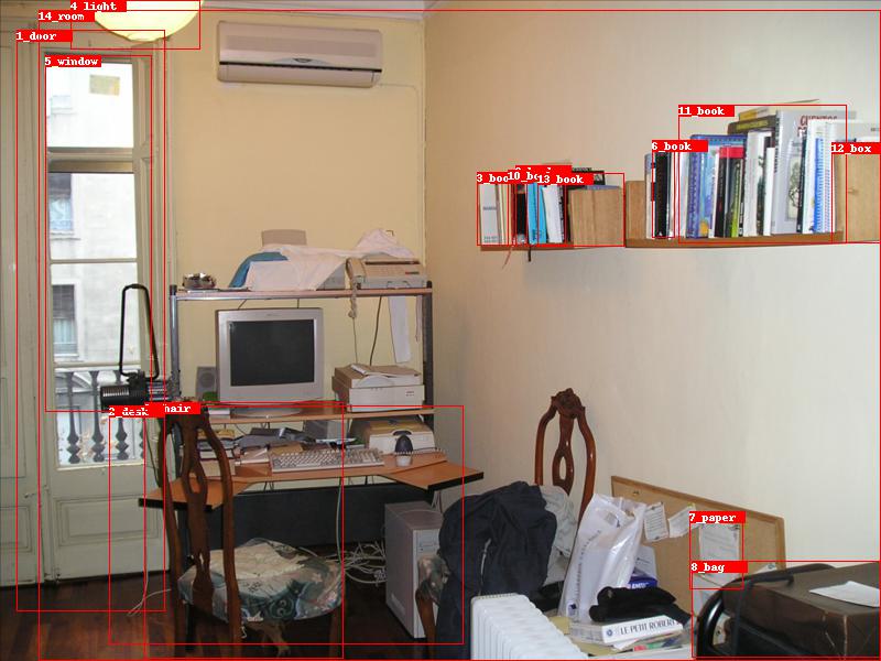
** Normal (Vanilia) argmax estimation **

**************************************************
rel_labels 0: 5_window => in => 14_room; score: 0.025266632437705994
rel_labels 1: 1_door => in => 14_room; score: 0.009757161140441895
rel_labels 2: 2_desk => in => 14_room; score: 0.009384681470692158
rel_labels 3: 0_chair => in => 14_room; score: 0.007233844138681889
rel_labels 4: 0_chair => near => 2_desk; score: 0.0034478071611374617
rel_labels 5: 5_window => on => 1_door; score: 0.0008813929744064808
rel_labels 6: 4_light => on => 1_door; score: 0.0007640126277692616
rel_labels 7: 4_light => in => 14_room; score: 0.0004628885071724653
rel_labels 8: 1_door => has => 5_window; score: 0.00039950464270077646
rel_labels 9: 12_box => in => 14_room; score: 0.0002094725496135652
rel_labels 10: 7_paper => on => 2_desk; score: 0.0001718419516691938
rel_labels 11: 3_book => on => 2_desk; score: 5.526307722902857e-05
rel_labels 12: 10_book => on => 2_desk; score: 4.91523023811169e-05
rel_labels 13: 11_book => in => 14_room; score: 4.17599621869158e-05
rel_labels 14: 13_book => in => 14_room; score: 2.9153519790270366e-05
rel_labels 15: 8_bag => on => 2_desk; score: 2.740809395618271e-05
rel_labels 16: 9_book => on => 2_desk; score: 2.630994094943162e-05
rel_labels 17: 6_book => in => 14_room; score: 1.9420620446908288e-05
rel_labels 18: 9_book => in => 14_room; score: 1.8823122445610352e-05
rel_labels 19: 10_book => in => 14_room; score: 1.7273092453251593e-05


** Our total direct effect casuality estimation **

**************************************************
rel_labels 0: 5_window => in => 14_room; score: 0.9316350817680359
rel_labels 1: 2_desk => in => 14_room; score: 0.9267702102661133
rel_labels 2: 1_door => in => 14_room; score: 0.868871808052063
rel_labels 3: 0_chair => in => 14_room; score: 0.8664298057556152
rel_labels 4: 12_box => in => 14_room; score: 0.8048514723777771
rel_labels 5: 0_chair => under => 4_light; score: 0.7975059747695923
rel_labels 6: 2_desk => under => 4_light; score: 0.7918913960456848
rel_labels 7: 13_book => in => 14_room; score: 0.7865951061248779
rel_labels 8: 8_bag => in => 14_room; score: 0.7771527171134949
rel_labels 9: 7_paper => in => 14_room; score: 0.7696521878242493
rel_labels 10: 0_chair => at => 2_desk; score: 0.7678285241127014
rel_labels 11: 6_book => in => 14_room; score: 0.7667400240898132
rel_labels 12: 10_book => in => 14_room; score: 0.7562098503112793
rel_labels 13: 9_book => in => 14_room; score: 0.755908727645874
rel_labels 14: 3_book => in => 14_room; score: 0.7499572038650513
rel_labels 15: 11_book => in => 14_room; score: 0.7362657785415649
rel_labels 16: 4_light => above => 2_desk; score: 0.6984441876411438
rel_labels 17: 4_light => above => 0_chair; score: 0.6705607175827026
rel_labels 18: 14_room => has => 5_window; score: 0.6420085430145264
rel_labels 19: 0_chair => in front of => 1_door; score: 0.6367448568344116
Homework 5
What assumptions have I made that are important to my inferences/conclusions?
I have made three assumptions: consistency, SUTVA, and exchangeability. The explanations are:
(a) Consistency. The potential outcome if we were to assign intervention \(X\) (object features) is exactly \(Y\) (object relationships in the scene), i.e. \(Y=Y(X)\).
(b) SUTVA (stable-unit value assumption). The mapping \(x \mapsto Y(x)\) is a well-defined function from \({X}\) to the set of random variables (i.e. real-valued measurable functions) defined on our probability space. Here \(x\) is object features.
(c) Exchangeability. Potential outcomes (object relationships) \(Y(x)\) are independent from the treatment assignment (here is object features) \(X\) for each \(x \in {X}\).
\[Y(x) \perp X, \quad x \in X\]The last one, assumption for the conditional exchangeability and backdoor adjustment is important:
\[Y(x) \perp X, \quad x \in X\]This is important because, in this way, we can not care about the confounder image feature \(I\). However, if \(Y\) is not randomized, this assumption is tenuous. Now we suspect an unmeasured variable \(I\) that is associated with both \(X\) and \(Y\).
What alternatives to estimation/implementation/identification are available to investigate the sensitivity of my conclusions/inferences to my assumptions?
In counterfactual reasoning, the important step is to represent the features of the counterfactual object. Here I use the average image features across the dataset as the counterfactual features. But we can also use other formats, such as using the zero vector or constant vectors (e.g. all values are 1) to replace the original counterfactual features. Through experiments, we found that zero vectors achieve slightly worse performance than the mean image feature vectors.
Besides, the scene graph generation methods usually follow a two-stage [Tang et al. 2020] paradigm. The first stage is object detection, which helps localize and perceive the objects. The second stage is the relationship prediction network. Both two parts can be replaced with new architectures. For example, we can replace the original Faster R-CNN [Ren et al. 2015] with more accurate object detectors, such as DETR [Carion et al. 2020]. Experiments show that with a better object detector, the object relationship prediction would be more accurate.
How would your inferences/conclusions change (if at all) if your assumptions were violated?
Here I will adopt the Rosenbaum sensitivity analysis for the unmeasured confounding \(I\). I will use choose a sensitivity parameter \(\Gamma:=\exp (\gamma)\) to get the two extreme bounds: p-value1 and p-value2.
Why do I choose Rosenbaum instead of the Since we are densely conducting causal inference for each of the object pairs, thus Manski and E-value would not be applicable here. This is because Manski and E-value are more treatment (statistical) oriented. In a single image, we do not have enough pairs to conduct partial identification: finding a range of values that a causal estimand takes in the presence of unmeasured confounder \(I\). A similar case happens in E-value, where \(R R_{A U}\) and \(R R_{U Y}\) would be hard to get.
Given the observed outcome \(Y(x, i, z)\) and the counterfactual outcome \(Y(\bar{x}, i, z)\), we can use the idea of Rosenbaum sensitivity analysis here. To be specific, let \(c=Y(\bar{x}, i, z)\), and \(b=Y(x, i, z)\).
Then assume \(C\) follows the following distribution:
\[C \sim \operatorname{Binomial}\left(b+c, \frac{1}{2}\right) \approx \operatorname{Normal}\left(\frac{b+c}{2}, \frac{(b+c)}{4}\right)\]Then we can get the p-value:
\[P\left(\left|C-\frac{b+c}{2}\right| \geq\left|c-\frac{b+c}{2}\right|\right):=\mathrm{p} \text {-value }\]For large \(C\):
\[C \sim \operatorname{Binomial}\left(b+c, \frac{1}{1+\exp (-\gamma)}\right) \approx \operatorname{Normal}\left(\frac{b+c}{1+\exp (-\gamma)}, \frac{(b+c) \exp (-\gamma)}{(1+\exp (-\gamma))^2}\right)\]Then
\[P\left(\left|C-\frac{b+c}{1+\exp (-\gamma)}\right| \geq\left|c-\frac{b+c}{1+\exp (-\gamma)}\right|\right):=\mathrm{p} \text {-value- } 1\]For small \(C\):
\[C \sim \operatorname{Binomial}\left(b+c, \frac{1}{1+\exp (\gamma)}\right) \approx \operatorname{Normal}\left(\frac{b+c}{1+\exp (\gamma)}, \frac{(b+c) \exp (\gamma)}{(1+\exp (\gamma))^2}\right)\]and
\[P\left(\left|C-\frac{b+c}{1+\exp (\gamma)}\right| \geq\left|c-\frac{b+c}{1+\exp (\gamma)}\right|\right):=\mathrm{p} \text {-value-2 }\]For example, in our appendix example, we care about the relationship:
5_window => in => 14_room

In this case, after inference with the deep neural network, we get \(c=Y(\bar{x}, i, z)=0.9569\), and \(b=Y(x, i, z)=0.0253\).
We use the same pseudo-code in Matlab to conduct analysis.
Note that we need to scale the logits in the neural network to fit our count-based approach.
def sensitivityanalysis_rosenbaum_scene_graph_generation(Gamma):

    % Rosenbaum sensitivity analysis (scene graph generation)


    % Build counts:
    c  = 0.9569;
    b  = 0.0253;
    % Scale it to fit the count-based approach.
    c= c*100;
    b= b*100;
    disp('ATE estimate: ')
    disp(c/(c+b))

    %----------------------------------
    % Unbiased case
    mn = (c+b)/2;
    sd = sqrt(c+b)/2;
    pvalue = ( 1 - normcdf( abs((c-mn)/sd) ) )*2;
    disp('p-value: ')
    disp(pvalue)

    % Upward biased case
    mn = (c+b)/(1+1/Gamma);
    sd = sqrt( (c+b)*(1/Gamma)/((1+1/Gamma)^2) );
    pvalue1 = ( 1 - normcdf( abs((c-mn)/sd) ) )*2;
    disp('p-value-1: ')
    disp(pvalue1)

    % Downward biased case
    mn = (c+b)/(1+Gamma);
    sd = sqrt( (c+b)*(Gamma)/((1+Gamma)^2) );
    pvalue2 = ( 1 - normcdf( abs((c-mn)/sd) ) )*2;
    disp('p-value-2: ')
    disp(pvalue2)
For the overall sensitivity analysis:
def sensitivityanalysis_rosenbaum_varyGamma_scene_graph_generation:
    % Sensitivity analysis Rosenbaum (scene graph generation)


    for m=1:51
        Gamma = 1 + (m-1)/10;
        sensitivityanalysis_rosenbaum_lungcancer;
        p(m,:) = [Gamma,pvalue1,pvalue,pvalue2];
    end

    PrettyFig
    Colors
    hold on
    plot(p(:,1),p(:,2),'Color',clr(2,:),'LineWidth',1.5)
    plot(p(:,1),p(:,3),'Color',clr(3,:),'LineWidth',1.5)
    plot(p(:,1),p(:,4),'Color',clr(4,:),'LineWidth',1.5)
    plot(p(:,1),p(:,4)*0+0.05,'--','Color',clr(1,:),'LineWidth',1.5)
    xlabel('\Gamma','FontWeight','bold')
    ylabel('p-value','FontWeight','bold')
    legend({'worst','actual','best'},'Location','northwest')
    print('sensitivityanalysis_rosenbaum_varyGamma_scene_graph_generation','-dpng','-r1000')
We can get the following figure:

As you can see, after adopting the sensitivity analysis, we can determine the largest \(\Gamma=11.6\) that can preserves a significant relationship between two target objects at the significance level of 0.05.
In words, two objects will still lead to a significant relationship whenever the unmeasured confounder does not increase or decrease the odds of assignment by a factor of 11.6, which means that this relationship is not sensitive to the confounder.
If we focus on another pair of objects:
0_chair => in => 14_room
In this case, after inference with the deep neural network, we get \(c=Y(\bar{x}, i, z)=0.9737\), and \(b=Y(x, i, z)=0.0072\).
Using the above code, we can get the following figure:
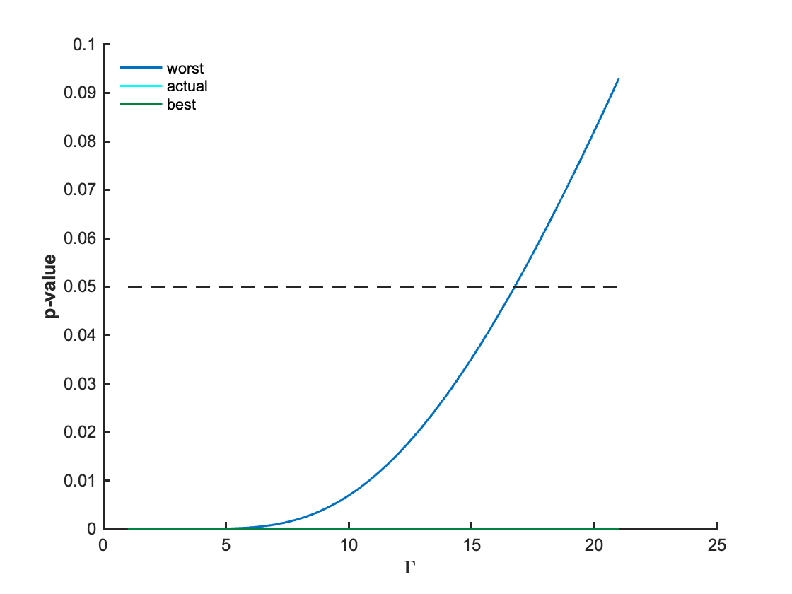
As you can see, after adopting the sensitivity analysis, we can determine largest \(\Gamma=16.7\) that can preserves a significant relationship between two target objects at the significance level of 0.05, meaning that our object relationship is not sensitive to unmeasured confounder \(I\).
From the above analysis, we know that such two object relationships are not sensitive to the unmeasured confounder.
But if my assumptions were violated, then it will show that the object relationship would be sensitive to the unmeasured confounder, where we need careful assumption/design of image feature \(I\).
What assumptions (if at all) cannot be investigated in any principled way?
We assume that the object detector is well-trained. However, there is no perfect object detector at all. For example, if a person is correctly localized using a bounding box, but misclassified as a “dog”, this will be extremely harmful to the result. But if this is the case, then the total direct effect would not work at all. The difficulty here is that in practice we have unlimited categories for objects, how can we precisely depict such sensitivity?
Homework 6
Remarks about my project
-
In summary, in this study, counterfactual reasoning is applied to alleviate the issue of biased visual object relationship prediction.
-
Our major finding is that causality modeling has shown its effectiveness in scene graph generation both quantitatively and qualitatively. As a result, the result in the scene graph is much more diverse and accurate.
-
Unfortunately, we were unable to address the issue of fully counterfactual modeling. That is to say, using the average image features across the dataset is not ideal to remove the target object while maintaining all other objects and background the same.
-
Possible avenues for future work include how to apply causality, in particular, counterfactual reasoning into recent vision-language foundation models. Recently, language pretrained models such as ChatGPT, DALLE-2, and CLIP are quickly changing the world, while they invariably include the bias from the training dataset. Therefore, an interesting question is, can causality help here?
-
This work is expected to contribute to the visual reasoning from a single image. The proposed approach is also helpful for the problem setting where bias naturally exists in the dataset.
References
- [Ren et al. 2015] Ren, Shaoqing, Kaiming He, Ross Girshick, and Jian Sun “Faster r-cnn: Towards real-time object detection with region proposal networks”, Advances in neural information processing systems 28 (2015)
- [Wang et al. 2020] Wang, Tan, Jianqiang Huang, Hanwang Zhang, and Qianru Sun “Visual commonsense r-cnn”, In Proceedings of the IEEE/CVF Conference on Computer Vision and Pattern Recognition, pp. 10760-10770. 2020
- [Tang et al. 2015] Tang, Kaihua, Yulei Niu, Jianqiang Huang, Jiaxin Shi, and Hanwang Zhang”Unbiased scene graph generation from biased training”, In Proceedings of the IEEE/CVF conference on computer vision and pattern recognition, pp. 3716-3725. 2020
-
[VanderWeele et al. 2013] VanderWeele, Tyler J “A three-way decomposition of a total effect into direct, indirect, and interactive effects“,Epidemiology (Cambridge, Mass.) 24, no. 2 (2013): 224.
-
[Krishna et al. 2017] Krishna, Ranjay, Yuke Zhu, Oliver Groth, Justin Johnson, Kenji Hata, Joshua Kravitz, Stephanie Chen et al. “Visual genome: Connecting language and vision using crowdsourced dense image annotations“,International journal of computer vision, 123(1), 32-73.
-
[He et al. 2017] He, Kaiming, Georgia Gkioxari, Piotr Dollár, and Ross Girshick. “Mask r-cnn”, In Proceedings of the IEEE international conference on computer vision, pp. 2961-2969. 2017.
- [Carion et al. 2017] Carion, Nicolas, Francisco Massa, Gabriel Synnaeve, Nicolas Usunier, Alexander Kirillov, and Sergey Zagoruyko. “End-to-end object detection with transformers”, In European conference on computer vision, pp. 213-229. Springer, Cham, 2020.