Prev: L2, Next: L4 , Assignment: A2 , Practice Questions: M6 M7 M8 , Links: Canvas, Piazza, Zoom, TopHat (453473)
Tools
📗 Calculator:
📗 Canvas:
pen
📗 You can expand all TopHat Quizzes and Discussions: , and print the notes: , or download all text areas as text file: .
# Unsupervised Learning
📗 Supervised learning: \(\left(x_{1}, y_{1}\right), \left(x_{2}, y_{2}\right), ..., \left(x_{n}, y_{n}\right)\).
📗 Unsupervised learning: \(\left(x_{1}\right), \left(x_{2}\right), ..., \left(x_{n}\right)\).
➩ Clustering: separates items into groups.
➩ Novelty (outlier) detection: finds items that are different (two groups).
➩ Dimensionality reduction: represents each item by a lower dimensional feature vector while maintaining key characteristics.
📗 Unsupervised learning applications:
➩ Google news.
➩ Google photo.
➩ Image segmentation.
➩ Text processing.
➩ Data visualization.
➩ Efficient storage.
➩ Noise removal.
# Hierarchical Clustering
➩ Start with each items as a cluster.
➩ Merge clusters that are closest to each other.
➩ Result in a binary tree with close clusters as children.
In-class Discussion
ID:📗 [1 points] Given the following dataset, use hierarchical clustering to divide the points into groups. Drag one point to another point to merge them into one cluster. Click on a point to move it out of the cluster.
# Distance between Points
📗 Distance between points in \(m\) dimensional space is usually measured by Euclidean distance (also called \(L_{2}\) distance).
➩ Euclidean distance (\(L_{2}\)): \(\left\|x_{i} - x_{j}\right\|_{2} = \sqrt{\left(x_{i 1} - x_{j 1}\right)^{2} + \left(x_{i 2} - x_{j 2}\right)^{2} + ... + \left(x_{i m} - x_{j m}\right)^{2}}\): Wikipedia.
📗 Distances can also be measured by \(L_{1}\) or \(L_{\infty}\) distances.
➩ Manhattan distance (\(L_{1}\)): \(\left\|x_{i} - x_{j}\right\|_{1} = \left| x_{i 1} - x_{j 1} \right| + \left| x_{i 2} - x_{j 2} \right| + ... + \left| x_{i m} - x_{j m} \right|\): Wikipedia.
➩ Chebyshev distance (\(L_{\infty}\)): \(\left\|x_{i} - x_{j}\right\|_{\infty} = \displaystyle\max\left\{\left| x_{i 1} - x_{j 1} \right|, \left| x_{i 2} - x_{j 2} \right|, ..., \left| x_{i m} - x_{j m} \right|\right\}\): Wikipedia
In-class Discussion
📗 [1 points] Move the green point so that it is within 100 pixels of the red point measured by the distance. Highlight the region containing all points within 100 pixels of the red point.
Distance:
# Distance between Clusters
📗 Distance between clusters (group of points) can be measured by single linkage distance, complete linkage distance, or average linkage distance.
➩ Single linkage distance: the shortest distance from any item in one cluster to any item in the other cluster: Wikipedia.
➩ Complete linkage distance: the longest distance from any item in one cluster to any item in the other cluster: Wikipedia.
➩ Average linkage distance: the average distance from any item in one cluster to any item in the other cluster (average of distances, not distance between averages): Wikipedia.
In-class Discussion
ID:📗 [1 points] Highlight the Euclidean distance between the two clusters (red and blue) measured by the linkage distance.
Distance:
In-class Quiz
(Past Exam Question) ID:📗 [4 points] You are given the distance table. Consider the next iteration of hierarchical agglomerative clustering (another name for the hierarchical clustering method we covered in the lectures) using linkage. What will the new values be in the resulting distance table corresponding to the new clusters? If you merge two columns (rows), put the new distances in the column (row) with the smaller index. For example, if you merge columns 2 and 4, the new column 2 should contain the new distances and column 4 should be removed, i.e. the columns and rows should be in the order (1), (2 and 4), (3), (5).
\(d\) =
📗 Answer (matrix with multiple lines, each line is a comma separated vector): .
# Number of Clusters
📗 The number of clusters should be chosen based on prior knowledge about the dataset.
📗 The algorithm can also stop merging as soon as all the between-cluster distances are larger than some fixed threshold.
📗 The binary tree generated by hierarachical clustering is often called dendrogram: Wikipedia.
# K Means Clustering
📗 K-means clustering (2-means, 3-means, ...) iteratively updates a fixed number of cluster centers: Link, Wikipedia.
➩ Start with K random cluster centers.
➩ Assign each item to its closest center.
➩ Update all cluster centers as the center of its items.
In-class Discussion
ID:📗 [1 points] Given the following dataset, use k-means clustering to divide the points into groups. Move the centers and click on the center to move it to the center of the points closest to the center.
Total distortion:
# Total Distortion
📗 K means clustering tries to minimize the total distances of all items to their cluster centers. The total distance is called total distortion or inertia.
📗 Suppose the cluster centers are \(c_{1}, c_{2}, ..., c_{K}\), and the cluster center for an item \(x_{i}\) is \(c\left(x_{i}\right)\) (one of \(c_{1}, c_{2}, ..., c_{K}\)), then the total distortion is \(\left\|x_{1} - c\left(x_{1}\right)\right\|_{2}^{2} + \left\|x_{2} - c\left(x_{2}\right)\right\|_{2}^{2} + ... + \left\|x_{n} - c\left(x_{n}\right)\right\|_{2}^{2}\).
Math Note
📗 The K means procedure is similar to the gradient descent method to minimize the total distortion: Wikipedia.
➩ The gradient of the total distortion with respect to the cluster centers is \(-2 \displaystyle\sum_{x : c\left(x\right) = c_{k}} \left(x - c_{k}\right)\), setting this to \(0\) to obtain the update step formula \(c_{k} = \dfrac{1}{n_{k}} \displaystyle\sum_{x: c\left(x\right) = c_{k}} x\), where \(n_{k}\) is the number of items that belongs to cluster \(k\), and the sum is over all items in cluster \(k\).
➩ One issue with some optimization algorithms like gradient descent is that they sometimes converge to local minima that are not the global minimum. This is also the case for K means clustering: Wikipedia.
📗 [1 points] Move the point and change the learning rate to see the derivatives (slope of tangent line) of the function \(x^{2}\). Find an initial point + learning rate combination so that gradient descent will not find the global minimum.
Point: 0
Learning rate: 0.5
Derivative: 0
Point found after gradient descent: 0
1 slider
In-class Quiz
(Past Exam Question) ID:📗 [3 points] Perform k-means clustering on six points: \(x_{1}\) = , \(x_{2}\) = , \(x_{3}\) = , \(x_{4}\) = , \(x_{5}\) = , \(x_{6}\) = . Initially the cluster centers are at \(c_{1}\) = , \(c_{2}\) = . Run k-means for one iteration (assign the points, update center once and reassign the points once). Break ties in distances by putting the point in the cluster with the smaller index (i.e. favor cluster 1). What is the reduction in total distortion? Use Euclidean distance and calculate the total distortion by summing the squares of the individual distances to the center.
📗 Note: the red points are the cluster centers and the other points are the training items.
📗 Answer: .
# Number of Clusters
📗 There are a few ways to choose the number of clusters K.
➩ K can be chosen based on prior knowledge about the items.
➩ K cannot be chosen by minimizing total distortion since the total distortion is always minimized at \(0\) when \(K = n\) (number of clusters = number of training items).
➩ K can be chosen by minimizing total distortion plus some regularizer, for example, \(c \cdot m K \log\left(n\right)\) where \(c\) is a fixed constant and \(m\) is the number of features for each item.
In-class Quiz
📗 [1 points] Upload an image and use K-means clustering to group the pixels into \(K\) clusters. Find an appropriate value of \(K\):
![]() 1. Click on the image to perform the clustering for iterations.
1. Click on the image to perform the clustering for iterations.
Number of clusters:
# Initial Clusters
📗 There are a few ways to initialize the clusters: Link.
➩ The initial cluster centers can be randomly chosen in the domain.
➩ The initial cluster centers can be randomly chosen as \(K\) distinct items.
➩ The first cluster center can be a random item, the second cluster center can be the item that is the farthest from the first item, the third cluster center can be the item that is the farthest from the first two items, ...
# Unsupervised Learning
📗 Supervised learning: \(\left(x_{1}, y_{1}\right), \left(x_{2}, y_{2}\right), ..., \left(x_{n}, y_{n}\right)\).
📗 Unsupervised learning: \(\left(x_{1}\right), \left(x_{2}\right), ..., \left(x_{n}\right)\).
➩ Clustering: separates items into groups.
➩ Novelty (outlier) detection: finds items that are different (two groups).
➩ Dimensionality reduction: represents each item by a lower dimensional feature vector while maintaining key characteristics.
📗 Unsupervised learning applications:
➩ Google news.
➩ Google photo.
➩ Image segmentation.
➩ Text processing.
➩ Data visualization.
➩ Efficient storage.
➩ Noise removal.
# High Dimensional Data
📗 Text and image data are usually high dimensional: Link.
➩ The number of features of bag of words representation is the size of the vocabulary.
➩ The number of features of pixel intensity features is the number of pixels of the images.
📗 Dimensionality reduction is a form of unsupervised learning since it does not require labeled training data.
# Principal Component Analysis
📗 Principal component analysis rotates the axes (\(x_{1}, x_{2}, ..., x_{m}\)) so that the first \(K\) new axes (\(u_{1}, u_{2}, ..., u_{K}\)) capture the directions of the greatest variability of the training data. The new axes are called principal components: Link, Wikipedia.
➩ Find the direction of the greatest variability, \(u_{1}\).
➩ Find the direction of the greatest variability that is orthogonal (perpendicular) to \(u_{1}\), say \(u_{2}\).
➩ Repeat until there are \(K\) such directions \(u_{1}, u_{2}, ..., u_{K}\).
In-class Discussion
ID:📗 [1 points] Given the following dataset, find the direction (click on the diagram below to change the direction) in which the variation is the largest.
Projected variance:
Direction:
Projected points:
In-class Discussion
ID:📗 [1 points] Given the following dataset, find the direction (click on the diagram below to change the direction) in which the variation is the largest.
Projected variance:
Direction:
Projected points:
# Geometry
📗 A vector \(u_{k}\) is a unit vector if it has length 1: \(\left\|u_{k}\right\|^{2} = u^\top_{k} u_{k} = u_{k 1}^{2} + u_{k 2}^{2} + ... + u_{k m}^{2} = 1\).
📗 Two vectors \(u_{j}, u_{k}\) are orthogonal (or uncorrelated) if \(u^\top_{j} u_{k} = u_{j 1} u_{k 1} + u_{j 2} u_{k 2} + ... + u_{j m} u_{k m} = 0\).
📗 The projection of \(x_{i}\) onto a unit vector \(u_{k}\) is \(\left(u^\top_{k} x_{i}\right) u_{k} = \left(u_{k 1} x_{i 1} + u_{k 2} x_{i 2} + ... + u_{k m} x_{i m}\right) u_{k}\) (it is a number \(u^\top_{k} x_{i}\) multiplied by a vector \(u_{k}\)). Since \(u_{k}\) is a unit vector, the length of the projection is \(u^\top_{k} x_{i}\).
Math Note
📗 The dot product between two vectors \(a = \left(a_{1}, a_{2}, ..., a_{m}\right)\) and \(b = \left(b_{1}, b_{2}, ..., b_{m}\right)\) is usually written as \(a \cdot b = a^\top b = \begin{bmatrix} a_{1} & a_{2} & ... & a_{m} \end{bmatrix} \begin{bmatrix} b_{1} \\ b_{2} \\ ... \\ b_{m} \end{bmatrix} = a_{1} b_{1} + a_{2} b_{2} + ... + a_{m} b_{m}\). In this course, to avoid confusion with scalar multiplication, the notation \(a^\top b\) will be used instead of \(a \cdot b\).
📗 If \(x_{i}\) is projected onto some vector \(u_{k}\) that is not a unit vector, then the formula for projection is \(\left(\dfrac{u^\top_{k} x_{i}}{u^\top_{k} u_{k}}\right) u_{k}\). Since for unit vector \(u_{k}\), \(u^\top_{k} u_{k} = 1\), the two formulas are equivalent.
In-class Discussion
📗 [1 points] Compute the projection of the red vector onto the blue vector (drag the tips of the red or blue arrow, the green arrow represents the projection).
Red vector: , blue vector: .
Unit red vector: , unit blue vector: .
Projection: , length of projection: .
# Statistics
📗 The (unbiased) estimate of the variance of \(x_{1}, x_{2}, ..., x_{n}\) in one dimensional space (\(m = 1\)) is \(\dfrac{1}{n - 1} \left(\left(x_{1} - \mu\right)^{2} + \left(x_{2} - \mu\right)^{2} + ... + \left(x_{n} - \mu\right)^{2}\right)\), where \(\mu\) is the estimate of the mean (average) or \(\mu = \dfrac{1}{n} \left(x_{1} + x_{2} + ... + x_{n}\right)\). The maximum likelihood estimate has \(\dfrac{1}{n}\) instead of \(\dfrac{1}{n-1}\).
📗 In higher dimensional space, the estimate of the variance is \(\dfrac{1}{n - 1} \left(\left(x_{1} - \mu\right)\left(x_{1} - \mu\right)^\top + \left(x_{2} - \mu\right)\left(x_{2} - \mu\right)^\top + ... + \left(x_{n} - \mu\right)\left(x_{n} - \mu\right)^\top\right)\). Note that \(\mu\) is an \(m\) dimensional vector, and each of the \(\left(x_{i} - \mu\right)\left(x_{i} - \mu\right)^\top\) is an \(m\) by \(m\) matrix, so the resulting variance estimate is a matrix called variance-covariance matrix.
📗 If \(\mu = 0\), then the projected variance of \(x_{1}, x_{2}, ..., x_{n}\) in the direction \(u_{k}\) can be computed by \(u^\top_{k} \Sigma u_{k}\) where \(\Sigma = \dfrac{1}{n - 1} X^\top X\), and \(X\) is the data matrix where row \(i\) is \(x_{i}\).
➩ If \(\mu \neq 0\), then \(X\) should be centered, that is, the mean of each column should be subtracted from each column.
Math Note
📗 The projected variance formula can be derived by \(u^\top_{k} \Sigma u_{k} = \dfrac{1}{n - 1} u^\top_{k} X^\top X u_{k} = \dfrac{1}{n - 1} \left(\left(u^\top_{k} x_{1}\right)^{2} + \left(u^\top_{k} x_{2}\right)^{2} + ... + \left(u^\top_{k} x_{n}\right)^{2}\right)\) which is the estimate of the variance of the projection of the data in the \(u_{k}\) direction.
# Principal Component Analysis
📗 The goal is to find the direction that maximizes the projected variance: \(\displaystyle\max_{u_{k}} u^\top_{k} \Sigma u_{k}\) subject to \(u^\top_{k} u_{k} = 1\).
➩ This constrained maximization problem has solution (local maxima) \(u_{k}\) that satisfies \(\Sigma u_{k} = \lambda u_{k}\), and by definition of eigenvalues, \(u_{k}\) is the eigenvector corresponding to the eigenvalue \(\lambda\) for the matrix \(\Sigma\): Wikipedia.
➩ At a solution, \(u^\top_{k} \Sigma u_{k} = u^\top_{k} \lambda u_{k} = \lambda u^\top_{k} u_{k} = \lambda\), which means, the larger the \(\lambda\), the larger the variability in the direction of \(u_{k}\).
➩ Therefore, if all eigenvalues of \(\Sigma\) are computed and sorted \(\lambda_{1} \geq \lambda_{2} \geq ... \geq \lambda_{m}\), then the corresponding eigenvectors are the principal components: \(u_{1}\) is the first principal component corresponding to the direction of the largest variability; \(u_{2}\) is the second principal component corresponding to the direction of the second largest variability orthogonal to \(u_{1}\), ...
In-class Quiz
(Past Exam Question) ID:📗 [3 points] Given the variance matrix \(\hat{\Sigma}\) = , what is the first principal component? Enter a unit vector.
📗 Answer (comma separated vector): .
# Number of Dimensions
📗 There are a few ways to choose the number of principal components \(K\).
➩ \(K\) can be selected based on prior knowledge or requirement (for example, \(K = 2, 3\) for visualization tasks).
➩ \(K\) can be the number of non-zero eigenvalues.
➩ \(K\) can be the number of eigenvalues that are larger than some threshold.
# Reduced Feature Space
📗 An original item is in the \(m\) dimensional feature space: \(x_{i} = \left(x_{i 1}, x_{i 2}, ..., x_{i m}\right)\).
📗 The new item is in the \(K\) dimensional space with basis \(u_{1}, u_{2}, ..., u_{k}\) has coordinates equal to the projected lengths of the original item: \(\left(u^\top_{1} x_{i}, u^\top_{2} x_{i}, ..., u^\top_{k} x_{i}\right)\).
📗 Other supervised learning algorithms can be applied on the new features.
In-class Quiz
(Past Exam Question) ID:📗 [2 points] You performed PCA (Principal Component Analysis) in \(\mathbb{R}^{3}\). If the first principal component is \(u_{1}\) = \(\approx\) and the second principal component is \(u_{2}\) = \(\approx\) . What is the new 2D coordinates (new features created by PCA) for the point \(x\) = ?
📗 In the diagram, the black axes are the original axes, the green axes are the PCA axes, the red vector is \(x\), the red point is the reconstruction \(\hat{x}\) using the PCA axes.
📗 Answer (comma separated vector): .
# Reconstruction
📗 The original item can be reconstructed using the principal components. If all \(m\) principal components are used, then the original item can be perfectly reconstructed: \(x_{i} = \left(u^\top_{1} x_{i}\right) u_{1} + \left(u^\top_{2} x_{i}\right) u_{2} + ... + \left(u^\top_{m} x_{i}\right) u_{m}\).
📗 The original item can be approximated by the first \(K\) principal components: \(x_{i} \approx \left(u^\top_{1} x_{i}\right) u_{1} + \left(u^\top_{2} x_{i}\right) u_{2} + ... + \left(u^\top_{K} x_{i}\right) u_{K}\).
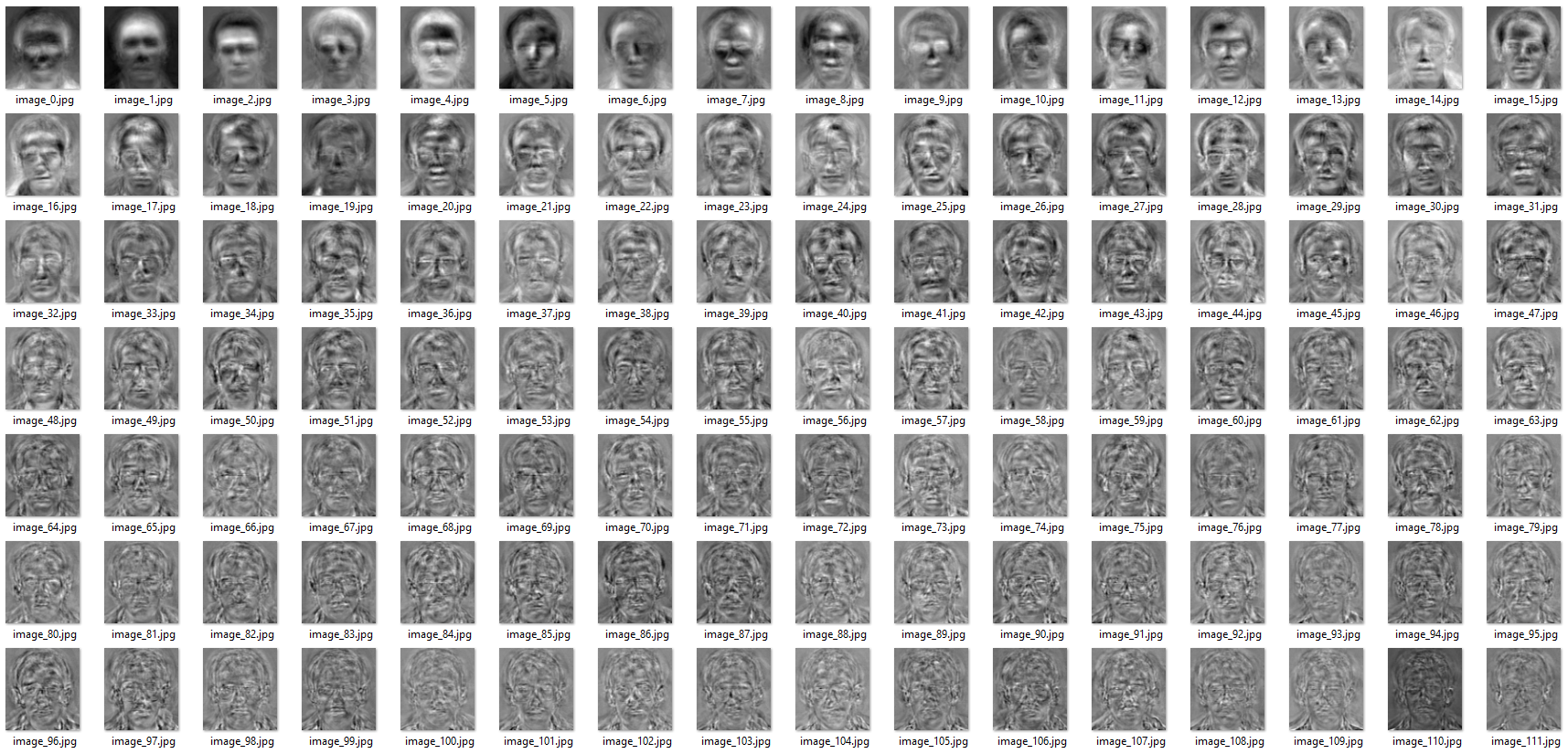
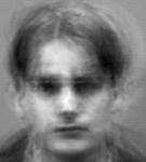
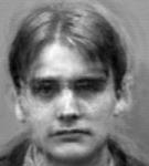
➩ Eigenfaces are eigenvectors of face images: every face can be written as a linear combination of eigenfaces. The first \(K\) eigenfaces and their coefficients can be used to determine and reconstruct specific faces: Link, Wikipedia.
Example
📗 An example of 111 eigenfaces:
📗 Reconstruction examples:
| K | Face 1 | Face 2 |
| 1 | 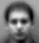
|
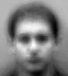
|
| 20 | 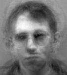
|
|
| 40 | 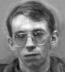
|
|
| 50 | 
|

|
| 80 | 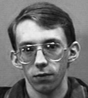
|
|
➩ Images by wellecks
# Non-linear PCA
📗 PCA features are linear in the original features.
📗 The kernel trick (used in support vector machines) can be used to first produce new features that are non-linear in the original features, then PCA can be applied to the new features: Wikipedia
➩ Dual optimization techniques can be used for kernels such as the RBF kernel which produces infinite number of new features.
📗 A neural network with both input and output being the features (no soft-max layer) is can be used for non-linear dimensionality reduction, called an auto-encoder: Wikipedia.
➩ The hidden units (\(K < m\) units, fewer than the number of input features) can be considered a lower dimensional representation of the original features.
test hi,di,li,ha,km,gd,kc,kg,pc,pt,pj,es,pn q
📗 Notes and code adapted from the course taught by Professors Jerry Zhu, Yingyu Liang, and Charles Dyer.
📗 Please use Ctrl+F5 or Shift+F5 or Shift+Command+R or Incognito mode or Private Browsing to refresh the cached JavaScript.
📗 Anonymous feedback can be submitted to: Form.
Prev: L2, Next: L4
Last Updated: June 27, 2026 at 9:07 PM