Prev: W6, Next: W8 , Practice Questions: M19 M20 , Links: Canvas, Piazza, Zoom, TopHat (744662)
Tools
📗 Calculator:
📗 Canvas:
pen
📗 You can expand all TopHat Quizzes and Discussions: , and print the notes: , or download all text areas as text file: .
# Computer Vision Tasks
📗 Unsupervised:
➩ Image segmentation.
📗 Supervised:
➩ Image colorization.
➩ Image reconstruction.
➩ Image synthesis.
➩ Image captioning.
➩ Object detection and tracking.
➩ Medical image analysis.
# Convolution
📗 Pixels are not independent of their neighbors. Ignoring the dependence is inappropriate for most computer vision tasks.
📗 Neighboring pixel intensities can be combined to create one feature that captures the information in the region around the pixel.
📗 Linearly combining pixels in a rectangular region is called convolution: Wikipedia.
➩ The convolution of an \(m \times m\) matrix (representing a training image indexed \(i\)) \(X_{i}\) with a \(\left(2 k + 1\right) \times \left(2 k + 1\right)\) filter \(W = \left[W_{s t}\right]_{s = -k, ..., k, t = -k, ..., k}\) is an \(m \times m\) matrix \(A_{i} = X_{i} \star W\), where the row \(r\) column \(c\) entry is given by \(\left[A_{i}\right]_{r c} = \displaystyle\sum_{s = -k}^{k} \displaystyle\sum_{t = -k}^{k} \left[X_{i}\right]_{r + t, c + s} W_{-s, -t}\).
➩ Technical note: the definition here flips the filter, for example the filter \(\begin{bmatrix} 1 & 2 & 3 \\ 4 & 5 & 6 \\ 7 & 8 & 9 \end{bmatrix}\) is flipped to \(\begin{bmatrix} 9 & 8 & 7 \\ 6 & 5 & 4 \\ 3 & 2 & 1 \end{bmatrix}\) before linear combination with the image. Similar linear combination without flipping the filter is called cross-correlation.
➩ The convolution filter is also called "kernel", but different from the kernel matrix for SVMs.
Math Note
📗 Convolution between two 1D vectors is also defined: the convolution of a vector \(x_{i} = \left(x_{i 1}, x_{i 2}, ..., x_{i m}\right)\) with a filter \(w = \left(w_{-k}, w_{-k + 1}, ..., w_{k-1}, w_{k}\right)\) is: \(a_{i} = \left(a_{i 1}, a_{i 2}, ..., a_{i m}\right) = x \star w\), where \(a_{i j} = w_{-k} x_{i \left(j + k\right)} + w_{-k + 1} x_{i \left(j + k - 1\right)} + ... + w_{k} x_{i \left(j - k\right)}\) for \(j = 1, 2, ..., m\).
📗 3D convolution can be defined in a similar way.
Example
In-class Discussion
📗 [1 points] Upload an image and try one of the following filters: . Image:
![]() 1. Click on the image to perform convolution with this filter: .
1. Click on the image to perform convolution with this filter: .
For Gaussian filter: size = , \(\sigma\) = . 0
In-class Quiz
ID:📗 [4 points] What is the convolution between the image and the filter using zero padding? Remember to flip the filter first.
📗 Answer (matrix with multiple lines, each line is a comma separated vector): .
Other students' answers:
# Traditional Computer Vision
📗 Traditional computer vision algorithms use engineered features for images based on image gradients.
➩ Image gradients are changes in pixel intensity due to the change in the location of the pixel: Wikipedia.
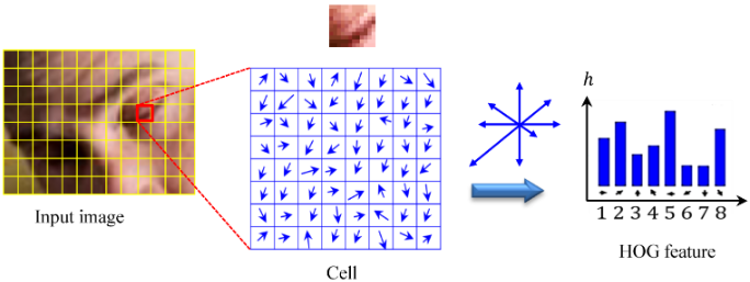
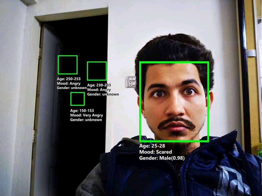
➩ Histogram of Gradients (HOG) can be used as a features for images and is often combined with SVM for face detection and recognition tasks: Wikipedia.
Math Note
📗 Image gradients can be computed (approximated) by convolution with the following filters: \(\nabla_{x} I = W_{x} \star I\) and \(\nabla_{y} I = W_{y} \star I\).
➩ (Discrete) derivative filter: \(W_{x} = \begin{bmatrix} -1 & 0 & 1 \\ -1 & 0 & 1 \\ -1 & 0 & 1 \end{bmatrix}\) and \(W_{y} = \begin{bmatrix} -1 & -1 & -1 \\ 0 & 0 & 0 \\ 1 & 1 & 1 \end{bmatrix}\).
➩ Sobel filters: \(W_{x} = \begin{bmatrix} -1 & 0 & 1 \\ -2 & 0 & 2 \\ -1 & 0 & 1 \end{bmatrix}\) and \(W_{y} = \begin{bmatrix} -1 & -2 & -1 \\ 0 & 0 & 0 \\ 1 & 2 & 1 \end{bmatrix}\), which can be viewed as a combination of the Gaussian filter (to blur the image) and the derivative filter: Wikipedia.
📗 Gradient magnitude at a pixel \((s, t)\) is given by \(G = \sqrt{\nabla_{x}^{2} I\left(s, t\right) + \nabla_{y}^{2} I\left(s, t\right)}\) and gradient direction \(\Theta = arctan\left(\dfrac{\nabla_{y} I\left(s, t\right)}{\nabla_{x} I\left(s, t\right)}\right)\).
Math Note
📗 For HOG features: in every 8 by 8 pixel region of an image, the gradient vectors \(\begin{bmatrix} \nabla_{x} I\left(s, t\right) \\ \nabla_{y} I\left(s, t\right) \end{bmatrix}\) are put into 9 orientation bins, for example, \(\left[0, \dfrac{2}{9} \pi\right], \left[\dfrac{2}{9} \pi, \dfrac{4}{9} \pi\right], ..., \left[\dfrac{16}{9} \pi, 2 \pi\right]\), and the histogram count is used as the HOG features.
📗 The resulting bins are normalized within a block of 2 by 2 regions.
📗 Scale Invariant Feature Transform (SIFT) produces similar feature representation using histogram of oriented gradients: Wikipedia.
➩ It is location invariant.
➩ It is scale invariant: images at different scales are used to compute the features.
➩ It is orientation invariant: dominant orientation in a larger region is calculated and all gradients in the region are rotated by the dominant orientation.
➩ It is illumination and contrast invariant: feature vectors are normalized so that they sum up to 1, and thresholded (values smaller than a threshold, for example 0.2, are made 0).
In-class Discussion
ID:📗 [1 points] Select the pixels in each of the 9 bins. The histogram is computed by summing up the .
1 0
# Haar Features
📗 HOG and SIFT features are too expensive to compute for real-time face detection tasks.
📗 Each image contains large number of locations at different scales, but faces only occur in very few of them.
📗 Each feature and classifier based on the feature should be easy to compute, and boosting can be used to combine simple features and classifiers.
📗 Haar features are differences between sums of pixel intensities in rectangular regions and can be obtained by convolution with filters such as \(\begin{bmatrix} 1 & 1 \\ -1 & -1 \end{bmatrix}\), \(\begin{bmatrix} 1 & -1 \\ 1 & -1 \end{bmatrix}\), ...: Wikipedia.
📗 Integral images (sum of pixel intensities above and to the left of every pixel) can be used to further speed up the computation: Wikipedia.
# Cascade Classifiers
📗 Each weak classifier can be a decision stump (decision tree with only one split) based on a Haar feature.
📗 Finding the threshold by comparing information gain is computationally expensive, so it is usually computed as the mid-point of the averages of the two classes.
📗 A sequence of weak classifiers can be combined into a strong classifier using AdaBoost (Adaptive Boosting).
➩ Start with a weak classifier and equal weights on all training items.
➩ Increase the weights on the items that are classified incorrectly, and train another weak classifier based on the updated weights.
➩ Continue the process to create a sequence of weak classifiers. The combined classifier is called a strong classifier.
📗 A sequence of strong classifiers can be combined into a cascade classifier.
➩ Start with a classifier with close to 100 percent detection rate by a possibly large false-positive rate.
➩ Train the next classifier still with close to 100 percent detection rate but with lower false-positive rate.
➩ Repeat this process to get a sequence of classifiers. The combined classifier called a cascade classifier.
Math Notes
📗 To create each classifier in the cascade classifier:
➩ Start by assigning equal weights for each image: \(w_{i} = \dfrac{1}{n}\) for \(i = 1, 2, ..., n\).
➩ Find optimal feature and threshold given the weights: the cost of mistake on image \(i\) should be weighted by \(w_{i}\), for example, \(C = C_{1} + C_{2} + ... + C_{n}\) where \(C_{i} = w_{i}\) if \(f_{j}\left(x_{i}\right) = y_{i}\) and \(C_{i} = 0\) otherwise.
➩ Choose weight of classifier \(f_{j}\) to be \(\alpha_{j} = \dfrac{1}{2} \log\left(\dfrac{1 - C}{C}\right)\).
➩ Update the weights to \(w_{i} = w_{i} \cdot e^{-y_{i} \alpha_{j} f_{j}\left(x_{i}\right)}\).
➩ Repeat the process until the desired detection rate and false positive rates are reached: the resulting classifier is \(\alpha_{1} f_{1} + \alpha_{2} f_{2} + ...\).
Example
# Viola Jones
📗 Viola Jones algorithm is a popular real-time face detection algorithm: Wikipedia.
➩ Each classifier operates on a 24 by 24 region of the image at multiple scales (scaling factor of 1.25).
➩ The regions can be overlapping. Nearby detection of faces are combined into a single detection.
# Learning Convolution
📗 The features can be engineered using computer vision techniques such as HOG or SIFT.
📗 They can also be learned as hidden units in a neural network. These neural networks are call convolutional neural networks (CNN): Link, Link, Wikipedia.
📗 Instead of activation units \(a = g\left(w^\top x + b\right)\) or \(a = g\left(w \cdot x + b\right)\), the dot product can be replaced by convolution (usually cross-correlation in practice, which is convolution without flipping the filters). The resulting matrix of activation units is called an activation map computed as \(A = g\left(W \star x + b\right)\).
➩ For filters in CNN, zero padding means adding zeros around the image pixel matrices so that the activation maps have the same size as the image; and no padding means not adding zeros around the image so the activation maps will be \(2 k\) pixels smaller than the image in each dimension.
➩ Filters with a stride of \(s\) means the skipping \(s - 1\) pixels when moving the filter around when computing the convolution: a stride of \(1\) is the standard convolution; and a stride of \(2 k + 1\) (filter size) is also called non-overlapping and each pixel is only used once in the computation of the convolution.
# Convolution and Pooling Layers
📗 Convolution can also be applied on activation maps in the previous layer \(A^{\left(l\right)} = g\left(W^{l} \star A^{\left(l - 1\right)} + b\right)\).
📗 Multiple units (in a \(k\) by \(k\) region) can be combined into one in pooling layers.
➩ Max pooling computes the maximum in a square region: \(\left[A^{\left(l\right)}\right]_{r c} = \displaystyle\max_{s = 0, 1, ..., k, t = 0, 1, ..., k} \left\{\left[A^{\left(l-1\right)}\right]_{r k + s, c k + t}\right\}\), where \(k\) is the pooling filter size.
➩ Average pooling computes the average in a square region: \(\left[A^{\left(l\right)}\right]_{r c} = \dfrac{1}{k^{2}} \displaystyle\sum_{s = 0}^{k} \displaystyle\sum_{t = 0}^{k} \left[A^{\left(l-1\right)}\right]_{r k + s, c k + t}\).
➩ The pooling layers usually have no padding and stride \(k\) (non-overlapping).
📗 The filter weights in convolution layers need to be trained using gradient descent. The pooling layer does not have weights that need to be trained.
➩ The gradient with respect to the weights in the convolution layers can be computed using convolution: \(\dfrac{\partial C}{\partial W} = X \star \dfrac{\partial C}{\partial A}\) and \(\dfrac{\partial C}{\partial X} = \text{rot} W \star \dfrac{\partial C}{\partial A}\), where \(\text{rot} W\) is the filter matrix rotated by 180 degrees (for example \(\begin{bmatrix} a & b \\ c & d \end{bmatrix}\) to \(\begin{bmatrix} d & c \\ b & a \end{bmatrix}\)).
➩ The gradient for the pooling layers is (i) for max pooling: \(1\) for the maximum input, 0 for other unit, (ii) for average pooling: \(\dfrac{1}{k^{2}}\) for each of the units in the \(k \times k\) region.
In-class Discussion
📗 [1 points] How many weights need to be trained in the following convolutional neural network? Click on a unit in an activation map to see the filter weights.
Input: 6
Conv layer filter size: 3
Pooling layer filter size: 2
Output layer: 3
1 slider
In-class Quiz
ID:📗 [4 points] A convolutional neural network has input image of size x that is connected to a convolutional layer that uses a x filter, zero padding of the image, and a stride of 1. There are activation maps. (Here, zero-padding implies that these activation maps have the same size as the input images.) The convolutional layer is then connected to a pooling layer that uses x max pooling, a stride of (non-overlapping, no padding) of the convolutional layer. The pooling layer is then fully connected to an output layer that contains output units. There are no hidden layers between the pooling layer and the output layer. How many different weights must be learned in this whole network, not including any bias.
📗 Answer: .
Other students' answers:
# Examples of Convolutional Neural Networks
📗 AlexNet is one of the earliest deep CNN architecture: Wikipedia.
📗 InceptionNet (GoogLeNet) introduced Inception module and auxiliary classifiers to improve training CNN with large number of layers: Link.
➩ 1 by 1 convolutions are used to reduce the number of activation maps.
➩ auxiliary classifiers are added so that the gradient in earlier layers does not become zero even when many of the weights in later layers are close to 0.
📗 ResNet introduces additional skip layer connections to improve training networking that are very deep: Wikipedia.
📗 U-Net also uses skip layer connections for image segmentation tasks: Wikipedia.
In-class Discussion
(Please wait for 5-10 seconds for the results ...)
➩ Top three:
➩ Predictions:
➩ Embeddings:
Other students' answers:
test fil,cv,hog,cnd,cnn,mn q
📗 Notes and code adapted from the course taught by Professors Jerry Zhu, Yingyu Liang, and Charles Dyer.
📗 Please use Ctrl+F5 or Shift+F5 or Shift+Command+R or Incognito mode or Private Browsing to refresh the cached JavaScript.
📗 If you missed the TopHat quiz questions, please submit the form: Form.
📗 Anonymous feedback can be submitted to: Form.
Prev: W6, Next: W8
Last Updated: June 27, 2026 at 9:07 PM