Prev: L10, Next: L12
Zoom: Link, TopHat: Link, GoogleForm: Link, Piazza: Link, Feedback: Link.
Tools
📗 You can expand all TopHat Quizzes and Discussions: , and print the notes: , or download all text areas as text file: .
📗 For visibility, you can resize all diagrams on page to have a maximum height that is percent of the screen height: .
📗 Calculator:
📗 Canvas:
pen
# Natural Language Processing Tasks
📗 Supervised learning:
➩ Speech recognition.
➩ Text to speech.
➩ Machine translation.
➩ Image captioning (combines with convolutional networks).
📗 Other similar sequential control or prediction problems:
➩ Handwritting recognition (online recognition: input is a sequence of pen positions, not an image).
➩ Time series prediction (for example, stock price prediction).
➩ Robot control (and other dynamic control tasks).
# Recurrent Networks
📗 Dynamic system uses the idea behind bigram models, and uses the same transition function over time:
➩ \(a_{t+1} = f_{a}\left(a_{t}, x_{t+1}\right)\) and \(y_{t+1} = f_{o}\left(a_{t+1}\right)\)
➩ \(a_{t+2} = f_{a}\left(a_{t+1}, x_{t+2}\right)\) and \(y_{t+2} = f_{o}\left(a_{t+2}\right)\)
➩ \(a_{t+3} = f_{a}\left(a_{t+2}, x_{t+3}\right)\) and \(y_{t+3} = f_{o}\left(a_{t+3}\right)\)
➩ ...
📗 Given input \(x_{i,t,j}\) for item \(i = 1, 2, ..., n\), time \(t = 1, 2, ..., t_{i}\), and feature \(j = 1, 2, ..., m\), the activations can be written as \(a_{t+1} = g\left(w^{\left(a\right)} \cdot a_{t} + w^{\left(x\right)} \cdot x_{t} + b^{\left(a\right)}\right)\).
➩ Each item can be a sequence with different number of elements \(t_{i}\), therefore, each item has different number of activation units \(a_{i,t}\), \(t = 1, 2, ..., t_{i}\).
➩ There can be either one output unit at the end of each item \(o = g\left(w^{\left(o\right)} \cdot a_{t_{i}} + b^{\left(o\right)}\right)\), or \(t_{i}\) output units one for each activation unit \(o_{t} = g\left(w^{\left(o\right)} \cdot a_{t} + b^{\left(o\right)}\right)\).
📗 Multiple recurrent layers can be added where the previous layer activation \(a^{\left(l-1\right)}_{t}\) can be used in place of \(x_{t}\) as the input of the next layer \(a^{\left(l\right)}_{t}\), meaning \(a^{\left(l\right)}_{t+1} = g\left(w^{\left(l\right)} \cdot a^{\left(l\right)}_{t} + w^{\left(l-1\right)} \cdot a^{\left(l-1\right)}_{t+1} + b^{\left(l\right)}\right)\).
📗 Neural networks containing recurrent units are called recurrent neural networks: Wikipedia.
➩ Convolutional layers share weights over different regions of an image.
➩ Recurrent layers share weights over different times (positions in a sequence).
In-class Discussion
📗 [1 points] Which weights (including copies of the same weight) are used in one backpropogation through time gradient descent step when computing \(\dfrac{\partial C}{\partial w^{\left(x\right)}}\)? Use the slider to unfold the network given an input sequence.
Input sequence length: 1
Output is also a sequence:
1 slider
# Backpropogation Through Time
📗 The gradient descent algorithm for recurrent networks are called Backpropagation Through Time (BPTT): Wikipedia.
📗 It computes the gradient by unfolding a recurrent neural network in time.
➩ In the case with one output unit at the end, \(\dfrac{\partial C_{i}}{\partial w^{\left(o\right)}} = \dfrac{\partial C_{i}}{\partial o_{i}} \dfrac{\partial o_{i}}{\partial w^{\left(o\right)}}\), and \(\dfrac{\partial C_{i}}{\partial w^{\left(a\right)}} = \dfrac{\partial C_{i}}{\partial o_{i}} \dfrac{\partial o_{i}}{\partial a_{t_{i}}} \dfrac{\partial a_{t_{i}}}{\partial w^{\left(a\right)}} + \dfrac{\partial C_{i}}{\partial o_{i}} \dfrac{\partial o_{i}}{\partial a_{t_{i}}} \dfrac{\partial a_{t_{i}}}{\partial a_{t_{i} - 1}} \dfrac{\partial a_{t_{i} - 1}}{\partial w^{\left(a\right)}} + ... + \dfrac{\partial C_{i}}{\partial o_{i}} \dfrac{\partial o_{i}}{\partial a_{t_{i}}} \dfrac{\partial a_{t_{i}}}{\partial a_{t_{i} - 1}} ... \dfrac{\partial a_{2}}{\partial a_{1}} \dfrac{\partial a_{1}}{\partial w^{\left(a\right)}}\), and \(\dfrac{\partial C_{i}}{\partial w^{\left(x\right)}} = \dfrac{\partial C_{i}}{\partial o_{i}} \dfrac{\partial o_{i}}{\partial a_{t_{i}}} \dfrac{\partial a_{t_{i}}}{\partial w^{\left(x\right)}} + \dfrac{\partial C_{i}}{\partial o_{i}} \dfrac{\partial o_{i}}{\partial a_{t_{i}}} \dfrac{\partial a_{t_{i}}}{\partial a_{t_{i} - 1}} \dfrac{\partial a_{t_{i} - 1}}{\partial w^{\left(x\right)}} + ... + \dfrac{\partial C_{i}}{\partial o_{i}} \dfrac{\partial o_{i}}{\partial a_{t_{i}}} \dfrac{\partial a_{t_{i}}}{\partial a_{t_{i} - 1}} ... \dfrac{\partial a_{2}}{\partial a_{1}} \dfrac{\partial a_{1}}{\partial w^{\left(x\right)}}\).
➩ The case with one output unit for each activation unit is similar.
In-class Discussion
📗 [1 points] Which weights (including copies of the same weight) are used in one backpropogation through time gradient descent step when computing \(\dfrac{\partial C}{\partial w^{\left(x\right)}}\)? Use the slider to unfold the network given an input sequence.
Input sequence length: 1
Output is also a sequence:
1 slider
# Vanishing and Exploding Gradient
📗 Vanishing gradient: if the weights are small, the gradient through many layers will shrink exponentially to \(0\).
📗 Exploding gradient: if the weights are large, the gradient through many layers will grow exponentially to \(\pm \infty\).
📗 In recurrent neural networks, if the sequences are long, the gradients can easily vanish or explode.
📗 In deep fully connected or convolutional networks, vanishing or exploding gradient is also a problem.
# Gated Recurrent Unit and Long Short Term Memory
📗 Gated hidden units can be added to keep track of memories: Link.
➩ Technically adding small weights will not lead to vanishing gradient like multiplying small weights, so hidden units can be added together.
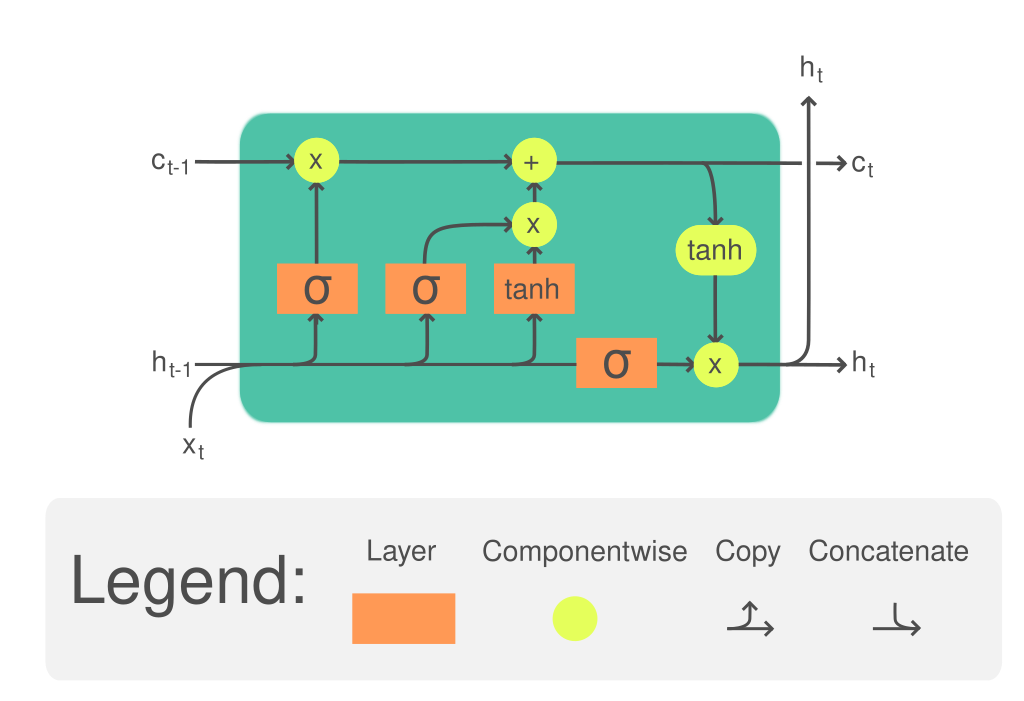
📗 Long Short Term Memory (LSTM): Wikipedia.
➩ The (long term) memory is updated by \(a^{\left(c\right)}_{t} = a^{\left(f\right)}_{t} \times a^{\left(c\right)}_{t-1} + a^{\left(i\right)}_{t} \times a^{\left(g\right)}_{t}\), where \(a^{\left(c\right)}\) is called the cell unit, \(a^{\left(f\right)}\) is the forget gate and controls how much memory to forget, \(a^{\left(i\right)}\) is the input gate and controls how much information to add to memory, \(a^{\left(g\right)}\) is the new values added to memory.
➩ The (short term memory) state is updated by \(a^{\left(h\right)} = a^{\left(o\right)} \times g\left(a^{\left(c\right)}_{t}\right)\), where \(a^{\left(h\right)}\) is the usual recurrent unit called hidden state, \(a^{\left(o\right)}\) is the output gate and controls how much information from the memory to reflect in the next state.
➩ Each of the gates are computed based on the hidden state and the input features (or the previous layer hidden states if there are multiple LSTM layers): \(a^{\left(f\right)}_{t} = g\left(w^{\left(f\right)} \cdot x_{t} + w^{\left(F\right)} \cdot a^{\left(h\right)}_{t-1} + b^{\left(f\right)}\right)\), \(a^{\left(i\right)}_{t} = g\left(w^{\left(i\right)} \cdot x_{t} + w^{\left(I\right)} \cdot a^{\left(h\right)}_{t-1} + b^{\left(i\right)}\right)\), \(a^{\left(g\right)}_{t} = g\left(w^{\left(g\right)} \cdot x_{t} + w^{\left(G\right)} \cdot a^{\left(h\right)}_{t-1} + b^{\left(g\right)}\right)\), \(a^{\left(o\right)}_{t} = g\left(w^{\left(o\right)} \cdot x_{t} + w^{\left(O\right)} \cdot a^{\left(h\right)}_{t-1} + b^{\left(o\right)}\right)\).
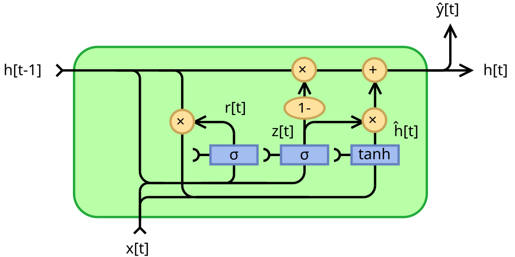
📗 Gated Recurrent Unit (GRU): Wikipedia.
➩ The memory is also updated through addition: \(a^{\left(h\right)}_{t} = \left(1 - a^{\left(z\right)}_{t}\right) \times a^{\left(h\right)}_{t-1} + a^{\left(z\right)}_{t} \times a^{\left(g\right)}_{t}\), where \(a^{\left(z\right)}\) is the update gate, and \(a^{\left(r\right)}\) is the reset gate.
➩ Each of the gates are computed in a similar way: \(a^{\left(z\right)}_{t} = g\left(w^{\left(z\right)} \cdot x_{t} + w^{\left(Z\right)} \cdot a^{\left(h\right)}_{t-1} + b^{\left(z\right)}\right)\), \(a^{\left(r\right)}_{t} = g\left(w^{\left(r\right)} \cdot x_{t} + w^{\left(R\right)} \cdot a^{\left(h\right)}_{t-1} + b^{\left(r\right)}\right)\), \(a^{\left(g\right)}_{t} = g\left(w^{\left(g\right)} \cdot x_{t} + w^{\left(G\right)} \cdot a^{\left(r\right)}_{t} \times a^{\left(h\right)}_{t-1} + b^{\left(g\right)}\right)\).
Example
📗 GRU:
📗 LTSM:
# Attention Mechanism
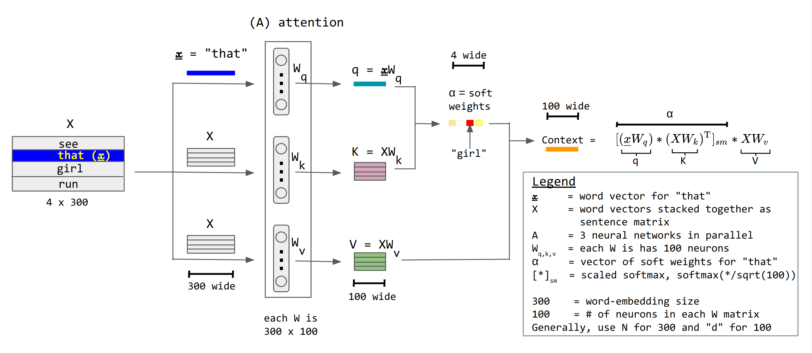
📗 Attention units keep track of which parts of the sentence is important and pay attention to, for example, scaled dot product attention units: Wikipedia.
➩ \(a^{\left(h\right)}_{t} = g\left(w^{\left(x\right)} \cdot x_{t} + b^{\left(x\right)}\right)\) is not recurrent.
➩ There are value units \(a^{\left(v\right)}_{t} = w^{\left(v\right)} \cdot a^{\left(h\right)}_{t}\), key units \(a^{\left(k\right)}_{t} = w^{\left(k\right)} \cdot a^{\left(h\right)}_{t}\), and query units \(a^{\left(q\right)}_{t} = w^{\left(q\right)} \cdot a^{\left(h\right)}_{t}\), and attention context can be computed as \(g\left(\dfrac{a^{\left(q\right)}_{s} \cdot a^{\left(k\right)}_{t}}{\sqrt{m}}\right) \cdot a^{\left(v\right)}_{t}\) where \(g\) is the softmax activation: here \(a^{\left(q\right)}_{s}\) represents the first word, \(a^{\left(k\right)}_{t}\) represents the second word, \(a^{\left(q\right)}_{s} \cdot a^{\left(k\right)}_{t}\) is the dot product (which represents the cosine of the angle between the two words, i.e. how similar or related the two words are), and \(a^{\left(v\right)}_{t}\) is the value of the second word to send to the next layer.
➩ The attention matrix is usually masked so that a unit \(a_{t}\) cannot pay attention to another unit in the future \(a_{t+1}, a_{t+2}, a_{t+3}, ...\) by making the \(a^{\left(q\right)}_{s} \cdot a^{\left(k\right)}_{t} = -\infty\) when \(s \geq t\) so that \(e^{a^{\left(q\right)}_{s} \cdot a^{\left(k\right)}_{t}} = 0\) when \(s \geq t\).
➩ There can be multiple parallel attention units called multi-head attention.
In-class Quiz
(Past Exam Question) ID:📗 [1 points] Compute the attention weights and the context value of the word with \(q_{i} = x_{i} \cdot w_{q}\) = ?
| Words | Key \(k_{j} = x_{j} \cdot w_{k}\) | Value \(v_{j} = x_{j} \cdot w_{v}\) | Attention Weights \(\alpha\) |
📗 Answer: .
In-class Quiz
(Past Exam Question) ID:📗 [1 points] Compute the attention weights and the context value of the word with \(q_{i} = x_{i} \cdot w_{q}\) = ?
| Words | Key \(k_{j} = x_{j} \cdot w_{k}\) | Value \(v_{j} = x_{j} \cdot w_{v}\) | Attention Weights \(\alpha\) |
| : | |||
| : | |||
| : | |||
| : |
📗 Answer: .
# Transformers
📗 Transformer is a neural network with attention mechanism and without reccurent units: Wikipedia.
📗 A transformer layer:
➩ Attention mechanism (multi-head attention).
➩ Feed-forward network.
➩ Residual connections.
📗 Tokenizer: convert between words and token IDs (integers), Link.
📗 Word embeddings: low dimensional vector representation of individual words (tokens).
➩ Word2vec: Wikipedia.
➩ Universal sentence encoder: Link.
📗 Positional encoding are used so that embedding vectors contain information about the word token and its position.
➩ Trained weights, or,
➩ Calculated by \(P\left(k, 2 i\right) = \sin\left(\dfrac{k}{n^{2 i / d}}\right)\) and \(P\left(k, 2 i + 1\right) = \cos\left(\dfrac{k}{n^{2 i / d}}\right)\) for word token \(k\) to position \(j \in \left\{2 i, 2 i + 1\right\}\) in the embedding vector: Link.
📗 Composite encoding = word embeddings + position embeddings.
➩ Attention mechanism produces contextual embeddings.
📗 Layer normalization trick is used so that means and variances of the units between attention layers and fully connected layers stay the same.
➩ Input \(a_{i}\), compute \(\mu_{x} = \dfrac{1}{d} \displaystyle\sum_{i=1}^{d} x_{i}\) and \(\sigma^{2}_{x} = \dfrac{1}{d} \displaystyle\sum_{i=1}^{d} \left(x_{i} - \mu_{x}\right)^{2}\).
➩ Output \(a^{\left(n\right)}_{i} = \dfrac{a_{i} - \mu_{x}}{\sqrt{\sigma^{2}_{x} + \varepsilon}}\), added \(\varepsilon\) small to prevent \(\sigma\) close to 0.
📗 Encoder-Decoder structure:
➩ Encoder: input sequence to a continuous representation \(z\) (useful for classification).
➩ Decoder: from \(z\), generate output sequence (useful for generation).
Example
From "Attention is All You Need":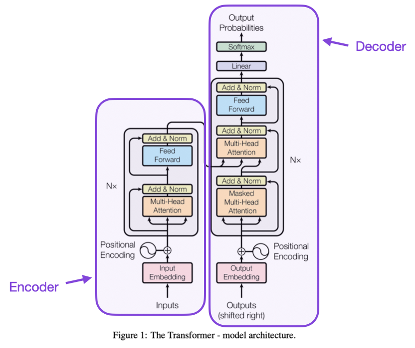
# Large Language Models
📗 GPT Series (Generative Pre-trained Transformer): Wikipedia.
➩ Pre-training: train all the weights on general purpose text dataset to learn contextualized word and sentence representations.
➩ Fine tuning for pre-trained decoder models freezes a subset of the weights (usually in earlier layers) and updates the other weights (usually the later layers) based on new datasets: Wikipedia.
📗 BERT (Bidirectional Encoder Representations from Transformers): Wikipedia.
➩ Fine tuning for pre-training encoder models adds task heads (additional layers at the end) and trains the weights in the task heads (sometimes also updates the pre-trained weights) for specific tasks.
📗 Many other large language models developed by different companies: Link.
➩ Prompt engineering does not alter the weights, and only provides more context (in the form of examples): Link, Wikipedia.
➩ Reinforcement learning from human feedback (RLHF) uses reinforcement learning techniques to update the model based on human feedback (in the form of rewards, and the model optimizes the reward instead of some form of costs): Wikipedia.
test rnn,bpt,ato,att q
📗 Notes and code adapted from the course taught by Professors Jerry Zhu, Yudong Chen, Yingyu Liang, and Charles Dyer.
📗 Content from note blocks marked "optional" and content from Wikipedia and other demo links are helpful for understanding the materials, but will not be explicitly tested on the exams.
📗 Please use Ctrl+F5 or Shift+F5 or Shift+Command+R or Incognito mode or Private Browsing to refresh the cached JavaScript.
📗 You can expand all TopHat Quizzes and Discussions: , and print the notes: , or download all text areas as text file: .
📗 If there is an issue with TopHat during the lectures, please submit your answers on paper (include your Wisc ID and answers) or this Google form Link at the end of the lecture.
📗 Anonymous feedback can be submitted to: Form. Non-anonymous feedback and questions can be posted on Piazza: Link
Prev: L10, Next: L12
Last Updated: June 27, 2026 at 9:07 PM