Prev: L21, Next: L23
Zoom: Link, Piazza: Link, Google Form: Link.
Wisc ID for in-class quiz: (if your wisc email is "test@wisc.edu", please enter "test")
Token: (will be given during the lectures)
22
id,answer_id;token,answer_check
# Markov Decision Process
📗 Reinforcement learning problem with multiple states is usually represented by Markov Decision Processes (MDP): Link, Wikipedia.
📗 Markov property on states and actions are assumed: \(\mathbb{P}\left\{s_{t+1} | s_{t}, a_{t}, s_{t-1}, a_{t-1}, ...\right\} = \mathbb{P}\left\{s_{t+1} | s_{t}, a_{t}\right\}\). The state in round \(t+1\), \(s_{t+1}\) only depends on the state and action in round \(t\), \(s_{t}\) and \(a_{t}\).
📗 The goal is learn a policy \(\pi\) to choose action \(\pi\left(s_{t}\right)\) that maximize the total expected discounted rewards: \(\mathbb{E}\left[r_{t} + \beta r_{t+1} + \beta^{2} r_{t+2} + ...\right]\).
➩ The reason a discount factor is used is so that the infinity sum is finite.
➩ Note that if the rewards are between \(0\) and \(1\), then the discounted total rewards is less than \(1 + \beta + \beta^{2} + ... = \dfrac{1}{1 - \beta}\).
Math Note
📗 To compute the sum, \(S = 1 + \beta + \beta^{2} + ...\), note that \(\beta S = \beta + \beta^{2} + \beta^{3} + ...\), so \(\left(1 - \beta\right) S = 1\) or \(S = \dfrac{1}{1 - \beta}\).
➩ This requires \(0 \leq \beta < 1\).
# Value Function
📗 The value function is the expected discounted reward given a policy function \(\pi\), or \(V^{\pi}\left(s_{t}\right) = \mathbb{E}\left[r_{t}\right] + \beta \mathbb{E}\left[r_{t+1}\right] + \beta^{2} \mathbb{E}\left[r_{t+2}\right] + ...\), where \(r_{t}\) is generated based on \(\pi\).
➩ To be precise, \(V^{\pi}\left(s_{t}\right) = \mathbb{E}\left[r_{t} | s_{t}, \pi\right] + \beta \mathbb{E}\left[r_{t+1} | s_{t}, \pi\right] + \beta^{2} \mathbb{E}\left[r_{t+2} | s_{t}, \pi\right] + ...\).
📗 The value function is the (only) function that satisfies the Bellman's equation: \(V^{\pi}\left(s_{t}\right) = \mathbb{E}\left[r_{t} | s_{t}, \pi\right] + \beta \mathbb{E}\left[V^{\pi}\left(s_{t+1}\right) | s_{t}, \pi\right]\).
📗 The optimal policy \(\pi^\star\) is the policy that maximizes the value function at every state.
# Q Function
📗 The Q function is the value function given a specific action in the current period (and follows \(\pi\) in future periods).
➩ By definition, \(Q^{\pi}\left(s_{t}, a_{t}\right) = \mathbb{E}\left[r_{t} | s_{t}, a_{t}\right] + \beta \mathbb{E}\left[r_{t+1} | s_{t}, a_{t}, \pi\right] + \beta^{2} \mathbb{E}\left[r_{t+2} | s_{t}, a_{t}, \pi\right] + ...\), which can be written as \(Q^{\pi}\left(s_{t}, a_{t}\right) = \mathbb{E}\left[r_{t} | s_{t}, a_{t}\right] + \beta \mathbb{E}\left[V^{\pi}\left(s_{t+1}\right) | s_{t}, a_{t}, \pi\right]\).
📗 Under the optimal policy, the Bellman's equation is satisfied: \(Q^\star\left(s_{t}, a_{t}\right) = \mathbb{E}\left[r_{t} | s_{t}, a_{t}\right] + \beta \mathbb{E}\left[V^\star\left(s_{t+1}\right) | s_{t}, a_{t}\right]\), for every state and action, where \(V^\star\left(s_{t+1}\right) = \displaystyle\max_{a} Q^\star\left(s_{t+1}, a\right)\).
📗 Bellman's equation can be used to iteratively solve for the Q function:
➩ Initialize \(\hat{Q}\left(s_{t}, a_{t}\right)\) for every state and action.
➩ Update \(\hat{Q}\left(s_{t}, a_{t}\right) \leftarrow \mathbb{E}\left[r_{t} | s_{t}, a_{t}\right] + \beta \mathbb{E}\left[\displaystyle\max_{a} \hat{Q}\left(s_{t+1}, a\right)\right]\).
➩ \(\hat{Q}\) converges to \(Q^\star\) given any initialization, assuming \(0 \leq \beta < 1\).
In-class Discussion
ID:📗 [1 points] Compute the optimal policy (at each state the car can go Up, Down, Left, Right, or Stay). The color represents the reward from moving to each state (more red means more negative and more blue means more positive). Click on the plot on the right to update the Q function once. The discount factor is .
📗 Q Function (columns are U, D, L, R, S):
📗 V Function:
📗 Policy:
In-class Quiz
(Past Exam Question) ID:📗 [4 points] Consider the following Markov Decision Process. It has two states \(s\), A and B. It has two actions \(a\): move and stay. The state transition is deterministic: "move" moves to the other state, while "stay" stays at the current state. The reward \(r\) is for move (from A and B), for stay (in A and B). Suppose the discount rate is \(\beta\) = .
Find the Q function in the format described by the following table. Enter a two by two matrix.
| State \ Action | stay | move |
| A | ? | ? |
| B | ? | ? |
📗 Answer (matrix with multiple lines, each line is a comma separated vector): .
# Q Learning
📗 The Q function can be learned by iteratively update the Q function using the Bellman's equation: Link, Wikipedia.
➩ \(\hat{Q}\left(s_{t}, a_{t}\right) = \left(1 - \alpha\right) \hat{Q}\left(s_{t}, a_{t}\right) + \alpha \left(r_{t} + \beta \displaystyle\max_{a} \hat{Q}\left(s_{t+1}, a\right)\right)\), where \(\alpha\) is the learning rate and is sometimes set to \(\dfrac{1}{1 + n\left(s_{t}, a_{t}\right)}\), \(n\left(s_{t}, a_{t}\right)\) is the number of visits to state \(s_{t}\) and action \(a_{t}\) in the past.
📗 Under certain assumptions, Q learning converges to the correct (optimal) Q function, and the optimal policy can be obtained by: \(\pi\left(s_{t}\right) = \mathop{\mathrm{argmax}}_{a} Q^\star\left(s_{t}, a\right)\) for every state.
In-class Discussion
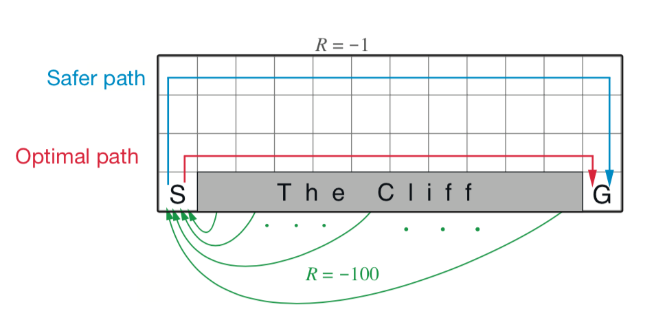
📗 [1 points] Compute the optimal policy (at each state the agent can go Up, Down, Left, Right). Falling into the cliff (black) leads to a loss of \(-100\) and walking (white) anywhere else leads to a loss of \(-1\). The agent starts at the blue tile and stops at the green tile.
📗 Click on the plot on the left to update the Q function times using Q learning. The plot on the right shows the number of visits to each square.
Epsilon greedy: \(\varepsilon\) = 0.1
Learning rate: \(\alpha\) = 0.1 or use \(\alpha = \dfrac{1}{1+n}\)
📗 Q Function (columns are U, D, L, R):
📗 V Function:
📗 Policy:
# SARSA
📗 An alternative to Q learning is SARSA (State Action Reward State Action). It uses a pre-specified action for the next period instead of the optimal action based on the current Q estimate: Wikipedia.
➩ \(\hat{Q}\left(s_{t}, a_{t}\right) = \left(1 - \alpha\right) \hat{Q}\left(s_{t}, a_{t}\right) + \alpha \left(r_{t} + \beta \hat{Q}\left(s_{t+1}, a_{t+1}\right)\right)\).
📗 The main difference is the action used in state \(s_{t+1}\).
➩ Q learning is an off-policy learning algorithm since \(a_{t+1}\) is the optimal policy in the next period, not a pre-specified policy (the Q function during learning does not correspond to any policy).
➩ SARSA is an on-policy learning algorithm since it computes the Q function based on a fixed policy.
In-class Discussion
📗 [1 points] Compute the optimal policy (at each state the agent can go Up, Down, Left, Right). Falling into the cliff (black) leads to a loss of \(-100\) and walking (white) anywhere else leads to a loss of \(-1\). The agent starts at the blue tile and stops at the green tile.
📗 Click on the plot on the left to update the Q function times using Q learning. The plot on the right shows the number of visits to each square.
Epsilon greedy: \(\varepsilon\) = 0.1
Learning rate: \(\alpha\) = 0.1 or use \(\alpha = \dfrac{1}{1+n}\)
📗 Q Function (columns are U, D, L, R):
📗 V Function:
📗 Policy:
# Exploration vs Exploitation
📗 The policy used to generate the data for Q learning or SARSA can be Epsilon Greedy or UCB (requires some modification for MDPs).
➩ Epsilon greedy: with probability \(\varepsilon\), \(a_{t}\) is chosen uniformly randomly among all actions; with probability \(1-\varepsilon\), \(a_{t} = \mathop{\mathrm{argmax}}_{a} \hat{Q}\left(s_{t}, a\right)\).
📗 The choice of action can be randomized too: \(\mathbb{P}\left\{a_{t} | s_{t}\right\} = \dfrac{c^{\hat{Q}\left(s_{t}, a_{t}\right)}}{c^{\hat{Q}\left(s_{t}, 1\right)} + c^{\hat{Q}\left(s_{t}, 2\right)} + ... + c^{\hat{Q}\left(s_{t}, K\right)}}\), where \(c\) is a parameter controlling the trade-off between exploration and exploitation.
# Questions?
📗 If you have questions, please use (i) Zoom chat, (ii) Piazza: Link, (iii) Office hours and discussion sessions. Please do NOT use Canvas mail and use email only to the course instructor (not TAs) for grading issues.
Additional In-class Discussion
📗 Sometimes a question not in the notes will be asked during the lecture, you can submit your answer here:
Notes (not visible to other students):
[Q1]
Submit your answer to see other students answers (click the submit button to refresh):
Additional In-class Quiz
📗 Sometimes a question not in the notes will be asked during the lecture, you can submit your answer here:
A. B.
C.
D.
E.
Notes (not visible to other students):
[Q2]
Submit your answer to see other students answers (click the submit button to refresh):
test car,ql,qcl,scl q https://script.google.com/macros/s/AKfycbyiidUAdiLc3YrKgOAM6T95ATulwDQxQilWVv1bK1L5sKRl8ozXfVs4PjCC2VtMWcIBpg/exec
# In-class Quiz Instructions
📗 To get full points on the in-class quizzes for a lecture:
➩ Submit relevant answers to the questions discussed during the lecture: incorrect answers are okay.
➩ Some questions require [notes] to earn the point.
➩ Some questions require special ID (given during the lecture) to earn the point.
➩ Do not submit answers to questions that are not discussed during the lectures. Each such submission will result in a deduction of one point.
➩ Submissions after the lecture, before the midterm (first 14 lectures) and the final exam (last 14 lectures), are accepted. After the exams, no in-class quiz submissions will be accepted.
➩ The grade on Canvas Assignment Q22 is computed as number of points divided by the number of questions asked (out of 1) and updated on Canvas every weekend.
📗 If there are any issues with submission on the website, please use this Google form: Link.
📗 Bonus point opportunities during a few lectures (added to in-class quiz above 20 points).
📗 Notes and code adapted from the course taught by Professors Jerry Zhu, Blerina Gkotse, Yudong Chen, Yingyu Liang, Charles Dyer. Some content are generated using Copilot .
Prev: L21, Next: L23
Last Updated: July 19, 2026 at 1:41 PM