Page Contents
Running the Compiler
The compiler is started with the following command:
java berkeley.cs.dmc.compiler.Main [-l logfile] <DynamicsSystem>
The <DynamicsSystem> is compiled class in the
CLASSPATH that implements
berkeley.cs.dmc.system.DynamicsSystem. The class must include
"System" somewhere in its name. The output file will have the same
name as the input class with "System" replaced by "Variable."
The logfile is the file where all messages will be
logged in addition to standard output. With or without this option
the compiler outputs a large amount of diagnositic text mostly to let
you know that the compiler is still churning away. Occasionally there
is useful text output in which case with a logfile you do not have to worry about it scrolling off the screen.
Compilation Phases
The DMC compiler has several phases it goes through when processing
a dynamical system. Each of the phase involves "learning" a specific
aspect of the dynamics systems, such as its long term or mid term
behavior. The compiler's diagnostic output shows the progress of the
compiler in each of the stages. Some of the compilation steps also
produce graphical output to give the user an idea of what the system
looks like and how the compiler is doing. This section explains each
of the phases and how to understand the diagnostic output.
Phase 1. Loading the System
In this phase, the system is loaded into the compiler and the general properties of the system are output. The example output in this documentation is produced from running the compiler on the TiltCarSystem included with in the DMC package.
Analysis started Wed Sep 30 01:01:58 PDT 1998 Class TiltCarSystem loaded. - numVariables = 2 - subsetLength = 2 - period = 3.076923076923077 - evaluationTechnique[0] = ITERATIVE - Cyclic true - evaluationTechnique[1] = FIRST_DERIVATIVE - Cyclic false |
Phase 2. Bounding
In the bounding system, the dynamics are run for a while to find the range of the system variables. The results of this phase are used in the rest of the compilation process.
RANGE[0] = -3.141592653589793 to 3.141592653589793 RANGE[1] = -4.20619925097702 to 3.5785218203207463 |
When this phase is complete, the bounds of all the variables is
output.
Phase 3. Finding the Equilibrium Distribution and Sampling Threshold
During this phase the dynamics systems's threshold for sampling is determined. This is defined as the time that must elapse while out of view before the object's state may be sampled from the equilibrium distribution.
Included in this phase is the calculation of the equlibrium distribution looks like. This calculation is done again by running the system for a while and tracking its positions.
SAMPLING THRESHOLD Maximum tree depth = 4 Building equilibrium distribution Generating initial conditions Dist 19999.003575000002 Dist 0.02219999999999999 Dist 0.01821666666666667 . . . Dist 0.0021931666666666766 Dist 0.002295384615384621 Dist 0.0019525641025641056 |
After the building the equibrium distribution a window with a picture of the equilibrium distribution is displayed.
The next step in this process is sampling a number of paths from the most commonly hit cells in the equilibrium distribution. The number of cells to test is displayed (in the example, 56), before the cell testing cells. Each cell is stepped forward until its distribution is sufficiently similar to the the equilibrium distribution. The median time for all of the cells to reach the equilibrium distribution is determined to be the final sampling threshold.
Will be testing 56 cells Cell 0 1 sub cells t = 3.076923076923077 : Dist 1.7500925925925928 t = 6.153846153846154 : Dist 1.862837037037037 t = 12.307692307692308 : Dist 1.8373074074074074 t = 24.615384615384617 : Dist 0.6996703703703704 t = 49.23076923076923 : Dist 0.29739074074074073 Cell -0.43663164469883037 2.0305812006020942 threshold is 49.23076923076923 . . . Cell 55 1 sub cells t = 3.076923076923077 : Dist 1.9749916666666667 t = 6.153846153846154 : Dist 1.749539814814815 t = 12.307692307692308 : Dist 1.086049074074074 t = 24.615384615384617 : Dist 0.5887518518518519 t = 49.23076923076923 : Dist 0.19254074074074073 Cell 2.4590657499646382 -1.6540518090728025 threshold is 49.23076923076923 Sampling threshold is: 49.23076923076923 |
During the process of testing the cells, another window similar to
the equilibrium distribution window displays the distribution of the
paths in each of the cells.
Phase 4. Training the Neural Network(s)
This is the final, and most time consuming stage of the compilation
process.
 This is also an incremental phase, meaning the longer this
phase runs the more accurate the produced dynamics variable will be.
For both these reasons, this phase has a early termination button that
when pressed will complete one more round of training and output the
compiled dynamics in its current state.
This is also an incremental phase, meaning the longer this
phase runs the more accurate the produced dynamics variable will be.
For both these reasons, this phase has a early termination button that
when pressed will complete one more round of training and output the
compiled dynamics in its current state.
The DMC compiler trains several neural networks corresponding to different time steps simultaneously. Each of the time steps will be displayed in the diagnostic output. The neural networks train for the change in position over a set timestep, so before the training can begin the bounds of the change is found for each time step.
After that the training begins, and continues until the error of the network is sufficiently low.
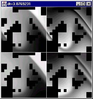
Learning, 3.076923076923077, 46.15384615384615 Time Steps: 3.076923076923077, 6.153846153846154, 12.307692307692308, 24.615384615384617 DELTA bounds for dt=3.076923076923077 [0] : -10.048204317334925 to 7.685835911195583 [1] : -5.744806528984153 to 5.977128556013383 DELTA bounds for dt=6.153846153846154 [0] : -16.75122312228373 to 14.470020287366076 [1] : -5.986710990524243 to 6.694725127409805 DELTA bounds for dt=12.307692307692308 [0] : -29.008618774608934 to 26.678529676408598 [1] : -6.658320841386993 to 6.605228483956829 DELTA bounds for dt=24.615384615384617 [0] : -50.65107934084002 to 51.67863539885129 [1] : -6.987734517298029 to 6.719370754816178 showing frame 0 showing frame 1 showing frame 2 showing frame 3 1-25000 Error (dt = 3.0769231): 0.04204621879589621 1-25000 Error (dt = 6.1538463): 0.04498558204896323 1-25000 Error (dt = 12.307693): 0.034458782135851816 1-25000 Error (dt = 24.615385): 0.025593887459391253 . . . 7750001-7775000 Error (dt = 3.0769231): 7.072306514990857E-4 7750001-7775000 Error (dt = 6.1538463): 0.004513747821680551 7750001-7775000 Error (dt = 12.307693): 0.008621666576673051 7750001-7775000 Error (dt = 24.615385): 0.009949576527785593 Done training. Analysis complete Wed Sep 30 04:24:19 PDT 1998 |
While training, a window for each timestep show the current state of the neural networks. Each window is divided into several sections, the upper area displays the actual system, and the lower area displays the neural networks approximation. The black squares corresponds to areas in where the dynamics system does not go.