CS 766 Computer
Vision, Spring 2017, Final Project
Image Colorization
Team Members : Srinivas Tunuguntla & Adithya Bhat
Introduction
This project explores the problem of adding colors a grayscale image. We intend to do this in a completely automated system, using Convolutional Neural Networks.
Previous Work
User Assisted
Scribble Based
- User provides scribbles that give reference colors.
- The system extends the colors to the rest of the image.
- However, the colors have to be given as input, they are not learnt.
Reference Based
- User provides reference image with similar features.
- The system transfers colors to similar regions to the given image.
- However, providing/selecting suitable reference images is vital to this method.
Automated
Feature Engineering Based
- Image features created via pre-processing.
- Feature engineering plays a major role.
- Machine Learning is used to map a feature vector to a color.
Neural Network Based
- Convolutional Neural Networks are the current state of the art.
- Machine Learning is used to learn both the features and the color schemes that map to a feature set.
- This is the approach we explore.
Dev Setup
Infrastructure
Google Cloud
Nvidia Tesla K80 GPU
Framework
Keras
Training Data
ImageNet
Geological Formation Synets
System Design
Color Space
Euclidean distance in the a-b space corresponds to visually perceived differences
L is the lightness channel
0 - black, 100 - white
a, b are color components
Range from -128 to +127 (or scaled to -100 to +100)
Problem Definition
Given a greyscale image(L channel), predict the color channel values a, b.
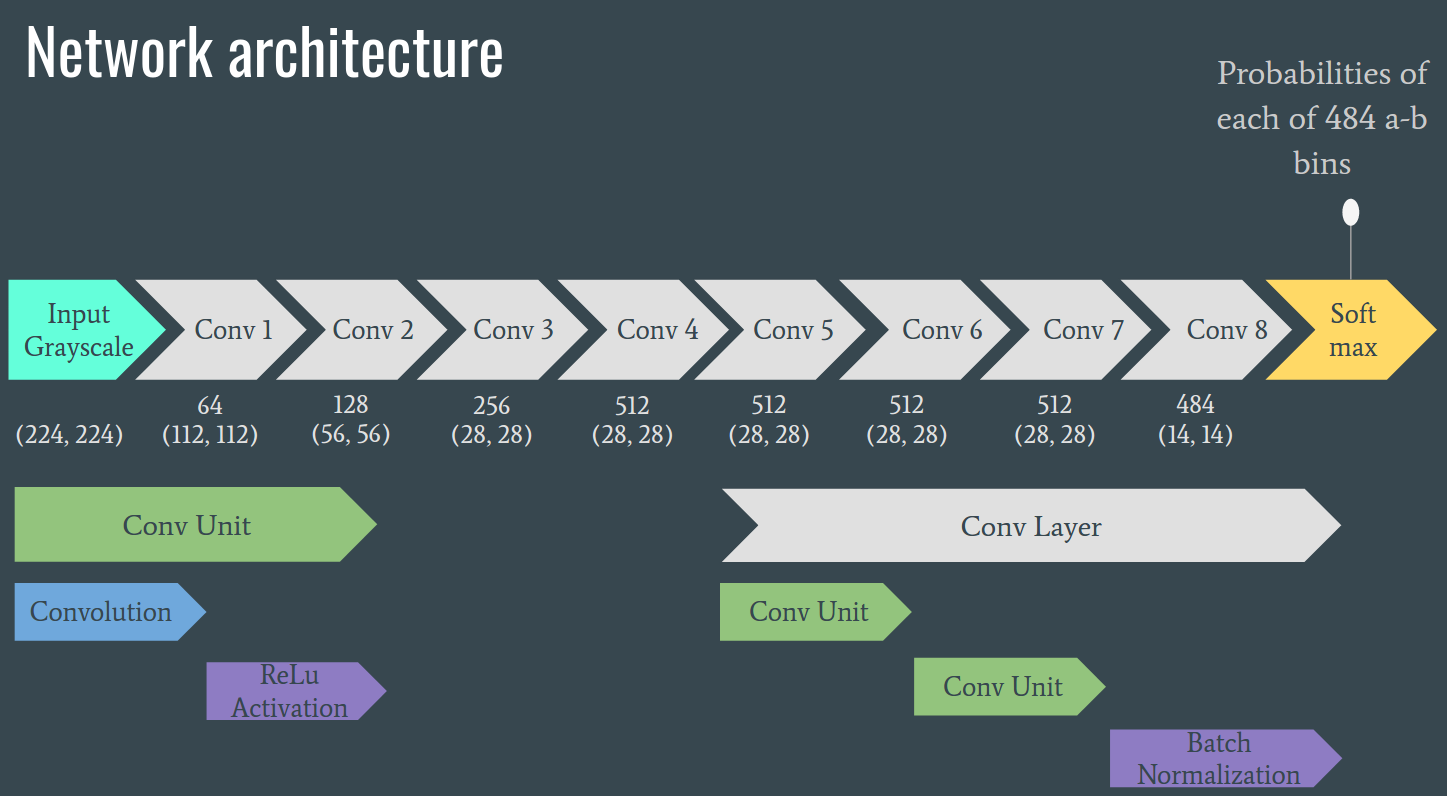
Network Architecture
Loss Function Design
Mean Squared Error
Mean squared error is the euclidean distance between the true a,b values and the predicted values. But, since the problem is inherently ambiguous (i.e. there are multiple valid colorizations), this loss function results in desaturated colorizations. This is because the model predicts the mean of all possible colorizations.
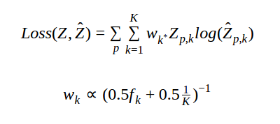
Multinomial Classification
To avoid desaturated colors, we formulate the problem as a multinomial classification over the a, b color space. The color space is divided into K bins and the model predicts a probability distribution over these bins. In our setting, we use K = 484 (22 bins for each channel a, b). To allow for multiple modes in the predicted probability distribution, we use the following loss function. 'Z' is the true bin index for pixel 'p' and '\hat{Z}' is the predicted bin.
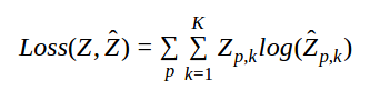
As long as there is a mode at the true value, the loss function above allows for multiple modes and hence allows multiple colorizations of the image.
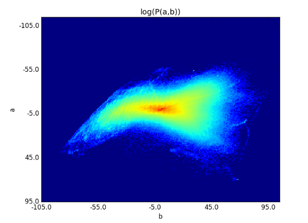
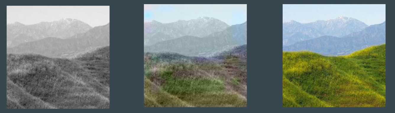
But, we noticed that the colorizations predicted by the model are biased towards low a,b values. This is because of the distribution of the colors present in our dataset. The distribution in our training set is shown below.
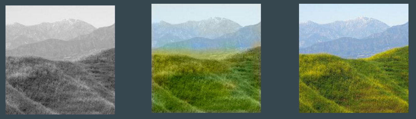
To encourage the model to use more vibrant colors we reweight each pixel loss based on the frequency of the true color of that pixel in the training set. The weight 'w' is inversely proportional to the frequency 'f'. The loss function is shown below.
Note:
the weights used are a knob that can be used to decide the trade-off between the vibrancy of the colors, and the realism of the colorization.
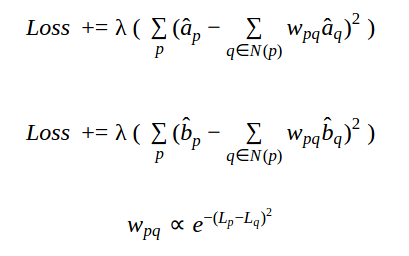
Segmentation
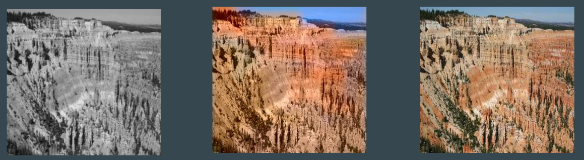
The loss function described above resulted in distinct patches of color over neighboring regions of an image. This is because, the colors for individual patches are predicted independently and the spatial information is not taken into account. Hence, we introduce spatial locality into the loss function. The intuition is that neighboring pixels with similar intensity tend to have similar colors. We calculate a weighted average of the colors of neighboring pixels and introduce a penalty term if the color of the current pixel is different from this calculated average. The weights for neighboring pixels depend on the similarities of intensities with the current pixel. The penalties for the a,b channels and the weight calculation are shown below. 'p' denotes the current pixel; N(p) denotes the neighborhood of the current pixel; L,a,b is the intensity and the color values of the pixel.
Results
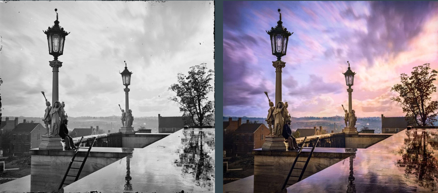
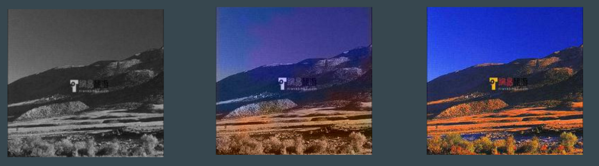
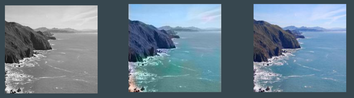
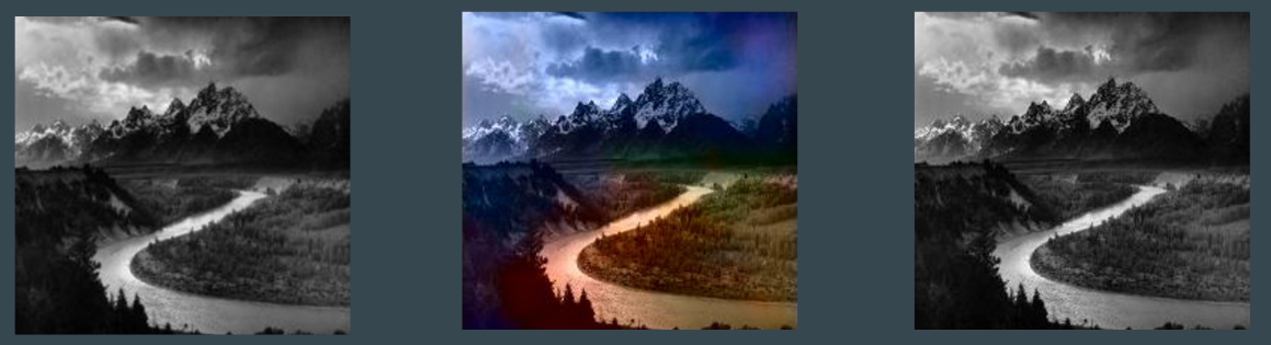
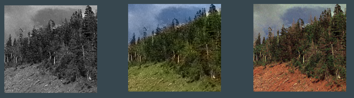
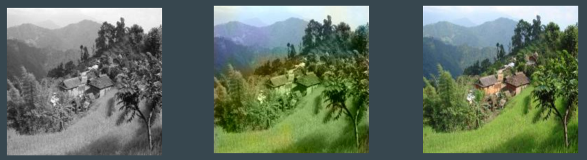
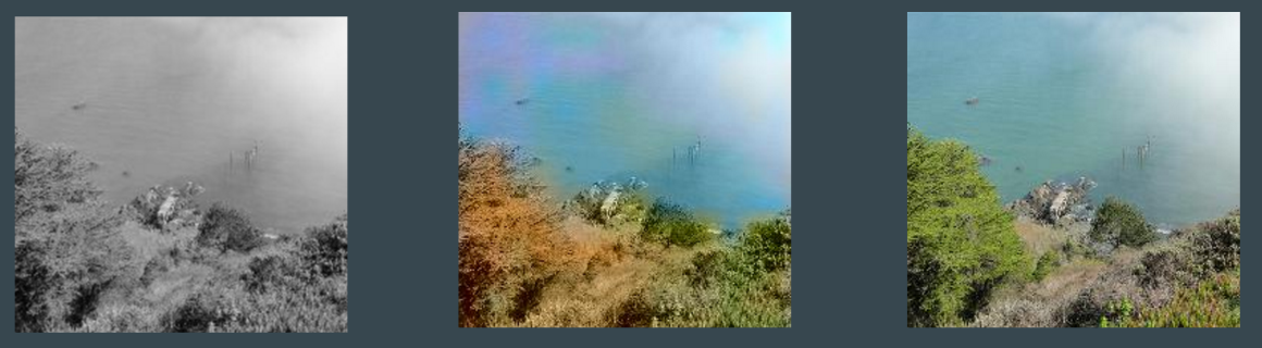
In all of the following results, the left image is the input grayscale image, the right image is the true colored image and the middle image is the predicted colorized image.
Before Rebalancing
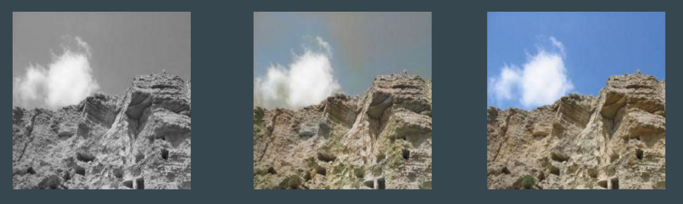
After Rebalancing
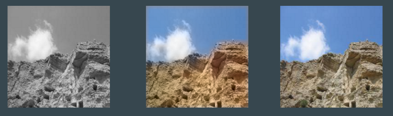
Before Segmentation
After Segmentation
Other Results
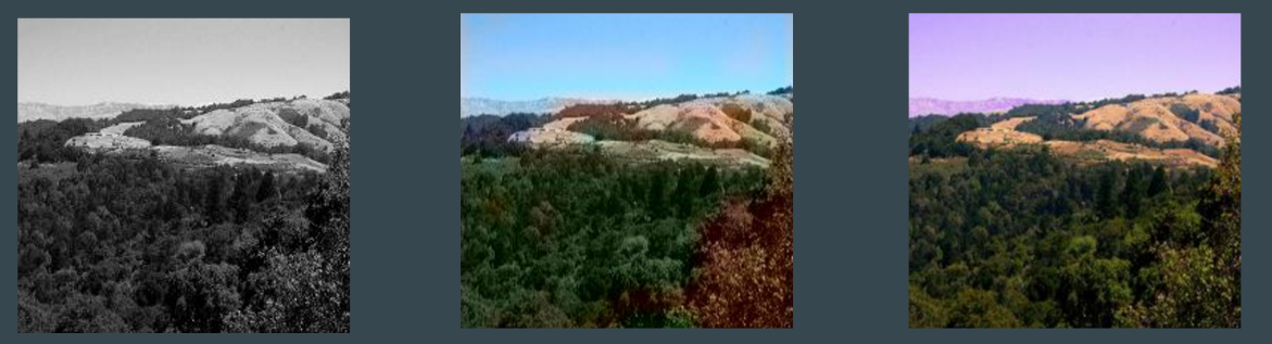
Failure Cases
Project Documents
Source Code
Github Repo
Project Proposal
Link
Mid Term Report
Link
Final Presentation
Link