Examples

1. Find the roots of the function

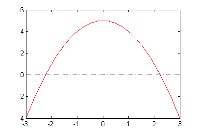
   First, plot the function. The range -3 to 3 will show the roots we are interested in.

   

   Place this code in a new m-file and run to see the plot shown here.

   % Find and plot the roots of y=-x^2+5 from -3 to 3
   
   % First, let's define an anonymous function to represent our function:
   fctn = @(x)-x.^2 + 5;  % element-wise for vector use (when plotting)
   
   xx = -3:0.1:3;
   yy = fctn(xx);  
   plot([-3 3],[0 0],'-.k', xx,yy,'r-') 
   

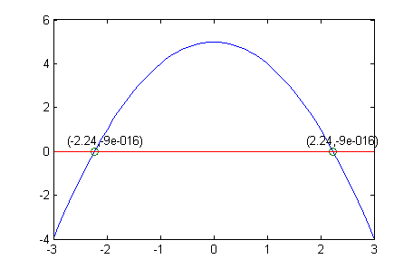
2. Use fzero to find the roots of the function in Example 1. Place this code in the same m-file as you created for Example 1:

   % Find the roots of the function y=-x^2+5 and save them in vectors x and y
   
   x0 = [-2 2];    % initial guesses for the roots
   
   x(1) = fzero(fctn,x0(1));  % find the 1st root and save it in x
   y(1) = fctn(x(1));         % evaluate at that root
   
   x(2) = fzero(fctn,x0(2));  % find the 2nd root and save it in x
   y(2) = fctn(x(2));         % evaluate at that root
   
   
   % Plot the function and the roots
   hold on
   plot( [-3 3],[0 0],'-.k', xx,yy,'r-' )  % plot y=0 and the curve
   
   % Display each root and a label for it on the plot
   plot( x, y, 'bo' )
   text( x(1)-0.5 , y(1)+0.5 , ...
        ['(' num2str(x(1),3) ',' num2str(y(1),1) ')' ])
   text(x(2)-0.5 , y(2)+0.5 , ...
        ['(' num2str(x(2),3) ',' num2str(y(2),1) ')' ])
   hold off
   

   Here is the figure that is produced, showing the curve and its roots.

   

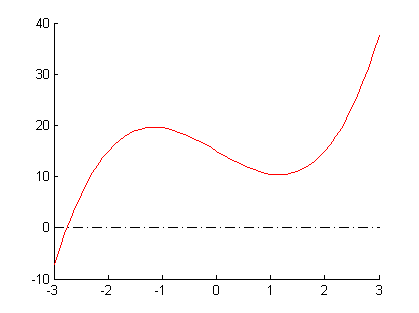
3. Find the roots of the function A plot of the function is shown for your convenience.

   

   This command will find the root near -3

       >> fzero( @(x)3/2*x.^3-6*x+15, -3 );