Exercises

Please complete each exercise or answer the question before reviewing the posted solution comments.

1. Find the roots of the following equation:

   First, enter the function into an M-file named "f1.m":

           function y = f1(x)
           y = x + 2.*exp(-x)-3;
         

   A general form of the command is:

   x = fzero(@function_name, x_value_guess or x range)

   To find our approximate x values, plot the function first. Create an M-file called f1plot.m and enter the following:

           xx=-5:.1:20;
           yy=f1(xx);
           plot(xx,yy)
           axis([-5 20 -5 20]);
           grid on
         

   Save and run f1plot.m. From the graph, you can see that there are two roots of the equation. They are near x = -1 and x = 3. To find the exact values, use the fzero routine:

           x1 = fzero(@f1,-1) or x1 = fzero(@f1, [-1,0])
           x2 = fzero(@f1,3)  or x2 = fzero(@f1, [2, 3])
         

   Matlab should come up with the exact values x1 = -0.5831 and x2 = 2.8887.

2. Write Matlab code that finds where the parabola (from Example 1) crosses the line y=3.

   To find where a function equals some value other than zero, use a function that subtracts the value from the function in question, and use fzero to find a root of the newly describe (or defined) function. A plot figure of the function is provided for your convenience.

   

   Copy the solution from Example 1 and make the changes that are shown in bold.

   % Exercise 1
   % Find and plot where y=-x^2+5 crosses the line y=3
   		  
   		  
   % First, let's define an anonymous function to represent our function:
   fctn = @(x)-x.^2 + 5;  % element-wise for vector use (when plotting)
   
   xx = -3:0.1:3;
   yy = fctn(xx);  
   plot([-3 3],[3 3],'-.k', xx,yy,'r-') 
   
   x0 = [-2 2];    % initial guesses for the roots
   
   x(1) = fzero(@(x)fctn(x)-3,x0(1));  % find where y=3
   y(1) = fctn(x(1));         % evaluate at that root
   
   x(2) = fzero(@(x)fctn(x)-3,x0(2));  % find where y=3
   y(2) = fctn(x(2));         % evaluate at that root
   
   hold on
   plot( [-3 3],[3 3],'-.k', xx,yy,'r-' )
   		  
   % Display each root and a label for it on the plot
   plot( x, y, 'bo' )
   text( x(1)-0.5 , y(1)+0.5 , ...
        ['(' num2str(x(1),3) ',' num2str(y(1),1) ')' ])
   text(x(2)-0.5 , y(2)+0.5 , ...
        ['(' num2str(x(2),3) ',' num2str(y(2),1) ')' ])
   hold off
           

   Note: the only change necessary was to subtract 3 from the function. The use of variables instead of many absolute values in the example code makes this possible. If you don't have example code to copy, these are the only commands necessary to find the x-values of the two points:

             >> x1 = fzero(@(x)fctn(x)-3,-2); % find negative x where y=3
             >> x1 = fzero(@(x)fctn(x)-3, 2); % find positive x where y=3
           

3. Approximate the data shown with a 7th degree polynomial and use fzero to find at what times (x-axis values) the temperature is 12 degrees. Plot your results.

               time=     0       2       4       6       8       10      12
               temp=  8.43    7.97    7.66    7.51    7.97    10.43   13.36
   
               time=    14      16      18      20      22       24
               temp= 15.39   15.71   14.61   12.28   10.59     9.82
             

   Hint: Incrementally develop your solution:

   1. Plot the data and the line temp=12.
   2. Compute and plot the 7th degree approximation.
   3. Add code to call fzero to get one of the time values.
   4. Plot the point to see if it looks right.
   5. Add code to call fzero to get the other time value.
   6. Plot this point also to see if it looks right.

   This code was incrementally developed as described above.

             clear;clc;
             time = [0	2	4	6	8	10	12	14	16	18	20	22	24];
             temp = [8.43	7.97	7.66	7.51	7.97	10.43	13.36	15.39	15.71	14.61	12.28	10.59	9.82];
   
             % Get coefficients of the 7th degree polynomial
             d = 7; % the degree of the approximating curve
             c = polyfit( time, temp, d );
             xx = 0:0.1:24;
             yy = polyval(c,xx);
   
             % 10 and 20 are approximate times when time will be 12 degrees
             t(1) = fzero( @(x)polyval(c,x)-12 , 10 );
             t(2) = fzero( @(x)polyval(c,x)-12 , 20 );
             y = polyval(c, t);
             disp(['Temp equals 12 degrees at time = ' num2str(t(1)) ' and time = ' num2str(t(2))]);
   
             % Plot it all
             hold on
             plot( xx, yy, 'r' );             % plot the approximation
             plot( [0 24], [12 12], 'k-.' );  % plot the line temp=12
             plot( time, temp, 'b*' );        % plot the data
             plot( t, y, 'go' )               % plot where curve intersect temp=12
             hold off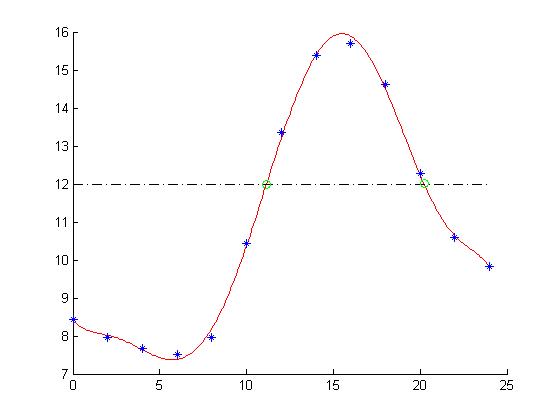
           

   

   The command window output is:

             
             Temp equals 12 degrees at time = 11.1454 and time = 20.2344