Examples

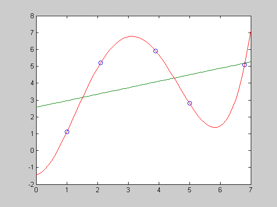
1. Given the data points, the following Matlab commands will compute the coefficients to interpolate the data with a 4th degree polynomial and compute the coefficients to approximate the data with a 1st degree polynomial and plot the results.

   clear; x = [1 2.1 3.9 5.0 6.8]; %Create data
y = [1.1 5.2 5.9 2.8 5.1];
c4 = polyfit(x,y,4);            % Interpolate data
c1 = polyfit(x,y,1);            % Approximate data
xx = 0.0:0.1:7;                 % x's to plot
yy4 = polyval(c4,xx);           % Interpolated y's
yy1 = polyval(c1,xx);           % Approximated y's
plot(x,y,'o',xx,yy1,xx,yy4)     % Plot the results


   

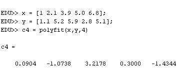
2. The following commands will compute the coefficients for the 4th degree polynomial that interpolates the given data and print them in the command window (because there is no ; at the end of the command.)

   x = [1 2.1 3.9 5.0 6.8];  % Create data
y = [1.1 5.2 5.9 2.8 5.1];
c4 = polyfit(x,y,4)       % Interpolate data


   

   
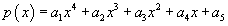
   where,
   
   Note the order in which polyfit returns the coefficients in the c4 vector. The first element c4(1)=0.0904 is the coefficient multiplying .

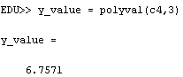
3. The following command will compute the value of the interpolation function at the point x=3.
   y_value = polyval(c4,3)