

Examples:
        e1 := x^2 → + 5*x + 6

        plot( e1, x=-5..5 )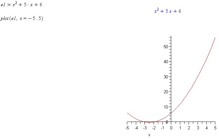
        e9 := x^2 → - x - 6

        plot( e9, x=-10..10 )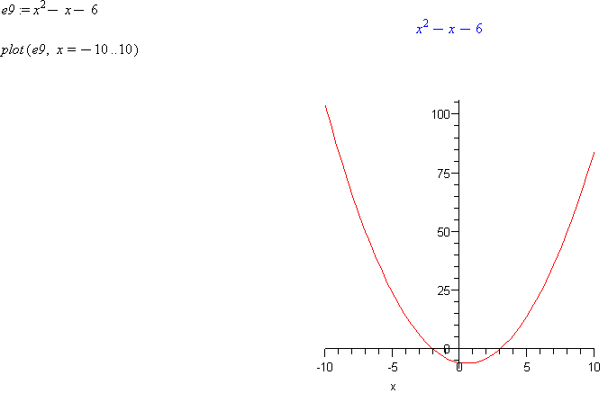
        e3:= tan(x)

        plot( e3, x=0..4 )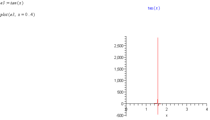
Comment: Note how the y axis has a very large value and this distorts the graph so that it is difficult to see what the function looks like.
plot(e3, x=0..4, y=-10..10)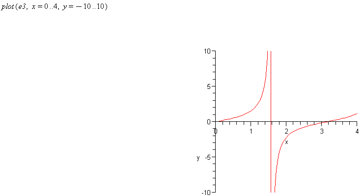
Comment: Note that the y axis can also be limited and this then produces a plot where it is easier to see the function. It is often necessary to scale the axes so that the resulting plot gives the information that you are seeking.
          eq10 := x^2 → + y^2 → = 6

          with(plots):

          implicitplot(eq10, x=-2.6..2.6, y=-2.6..2.6)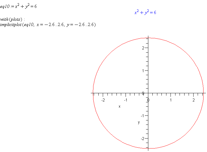
          eq11 := x^(3/2)*ln(x) - 7 = 0

          ex11 := lhs(eq11)

          plot(ex11, x=0..10)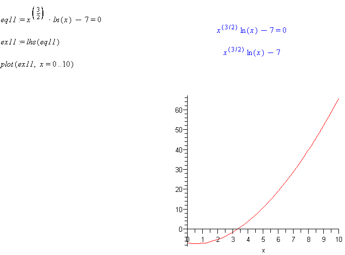
Comment: Note approximately where the function crosses the x-axis. This is the root of this equation.
Using the same worksheet as for example 6...
fsolve(eq11)
Comment: The best way to numerically find the roots of an equation is to first plot the equation to see approximately where the roots lie. Then use fsolve to find the roots.