Exercises
-
Solve the ODE:
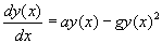 with a=5 and g=0.1. However, solve the ODE with the intial condition y(0)=100 and then solve with the initial condition y(0)=10.
Then plot both solutions on an appropriate time scale(x) to see the steady state behavior of both solutions on the same plot.
with a=5 and g=0.1. However, solve the ODE with the intial condition y(0)=100 and then solve with the initial condition y(0)=10.
Then plot both solutions on an appropriate time scale(x) to see the steady state behavior of both solutions on the same plot.
          ODE1:=diff(y(x), x) = a*y(x)-g*y(x)^2

          ODE2:=subs(a=5, g=0.1, ODE1)

          sol1:=dsolve({ODE2, y(0)=100}, y(x))

          sol2:=dsolve({ODE2, y(0)=10}, y(x))

          plot([rhs(sol1), rhs(sol2)], x=0..1.5, color=[red,blue])