Exercises
-
Using Euler's method and a time step of h=1, compute the first ten values of the solution of this ODE:

Step	 tk     tk+1     yk        F(tk,yk)  yk+1

   1     0      1.0     1.0       3.0       4.0

   2     1.0    2.0     4.0       6.0      10.0

   3     2.0    3.0    10.0000    9.4868   19.4868

   4     3.0    4.0    19.4868   13.2432   32.7300

   5     4.0    5.0    32.7300   17.1630   49.8930

   6     5.0    6.0    49.8930   21.1905   71.0835

   7     6.0    7.0    71.0835   25.2933   96.3769

   8     7.0    8.0    96.3769   29.4515  125.8284

   9     8.0    9.0   125.8284   33.6520  159.4804

  10     9.0   10.0   159.4804   37.8857  197.3660
-
Using Euler's method and a time step of h=0.1, compute the first three values of the solution of the ODE:

Step tk tk+1 yk F(tk,yk) yk+1 1 0 0.1 1.0000 3.0000 1.3000 2 0.1 0.2 1.3000 3.4205 1.6421 3 0.2 0.3 1.6421 3.8443 2.0265 4 0.3 0.4 2.0265 4.2706 2.4535 5 0.4 0.5 2.4535 4.6991 2.9235 6 0.5 0.6 2.9235 5.1294 3.4364 7 0.6 0.7 3.4364 5.5613 3.9925 8 0.7 0.8 3.9925 5.9944 4.5920 9 0.8 0.9 4.5920 6.4287 5.2348 10 0.9 1.0 5.2348 6.8639 5.9212 11 1.0 1.1 5.9212 7.3001 6.6512 -
Using Euler's method and a time step of h=10-2, compute the first three values of the solution of this ODE:

Step	 tk     tk+1     yk        F(tk,yk)  yk+1

   1     0      0.01    1         3         1.03
   2     0.01   0.02    1.03      3.044667  1.060446
   3     0.02   0.03    1.060446  3.089339  1.091340
-
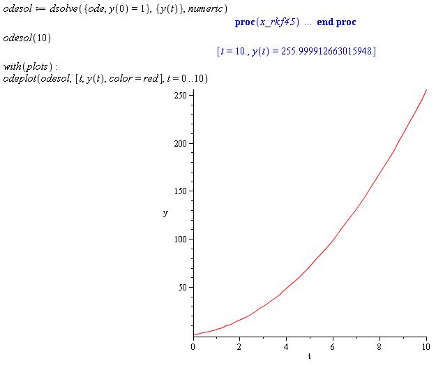
Now, use Maple to numerically solve this ODE in Maple and compare the accuracy of the Euler's approximations with the results that Maple's
dsolvecommand produces.
This is a simple application of Maple's dsolve command. Just be sure to include the correct initial condition and test your solution at various values of t before trying to plot the solution.

Notice that we can get much further in time with a few Maple commands than we ever could computing the values by hand. Even more importantly, the numeric approximation algorithm that Maple uses to compute the solution points is much more accurate than Euler's. It is 4th order or higher compared to first order for Euler's method.
The improved accuracy has to do with increased accuracy for smaller time steps. It may not be very evident when our first few approximations have relatively small time increments, but as we compute additional approximations further and further away in time from our initial condition or we increase our step size, the error in Euler's method no longer is no longer accepable to the smaller error of a 4th order (or higher) algorithm like Runge-Kutte.
See the help information on the
dsolvecommand for more information about the choice of numeric ODE solution algorithms that are readily available to you in Maple'sdsolvecommand.

