Prev: L40, Next: L42
# Lecture
📗 The lecture is in person, but you can join Zoom: 8:50-9:40 or 11:00-11:50. Zoom recordings can be viewed on Canvas -> Zoom -> Cloud Recordings. They will be moved to Kaltura over the weekends.
📗 The in-class (participation) quizzes should be submitted on TopHat (Code:741565), but you can submit your answers through Form at the end of the lectures too.
📗 The Python notebooks used during the lectures can also be found on: GitHub. They will be updated weekly.
# Lecture Notes
TopHat Game Again
➩ There will be 20 questions on the exam, 10 of them from past exams and quizzes, and 10 of them new questions (see Link for details). I will post \(n\) more questions next Monday that are identical or similar to \(n\) of the new questions on exam.
➩ A: \(n = 0\)
➩ B: \(n = 1\) if more than 50 percent of you choose B.
➩ C: \(n = 2\) if more than 75 percent of you choose C.
➩ D: \(n = 3\) if more than 95 percent of you choose D.
➩ E: \(n = 0\)
📗 Dimensionality Reduction
➩ Dimensionality reduction finds a low dimensional representation of a high dimensional point (item) in a way that points that close to each other in the original space are close to each other in the low dimensional space.
➩ Text and image data have a large number of features (dimensions), dimensionality reduction techniques can be used for visualization and efficient storage of these data types: Link.
Principal Component Analysis
➩ Principal component analysis finds the orthogonal directions that capture the highest variation, called principal components, and project the feature vectors onto the subspace generated by the principal components: Link.
📗 Projection
➩ A unit vector \(u\) in the direction of a vector \(v\) is \(u = \dfrac{v}{\left\|v\right\|}\), where \(\left\|v\right\| = \sqrt{v_{1}^{2} + v_{2}^{2} + ... v_{m}^{2}}\). Every unit vector satisfy \(u^\top u = 1\).
➩ The projection of a feature vector \(x\) onto the direction of a unit vector \(u\) is \(u^\top x\).
➩ Geometrically, the projection of \(x\) onto \(u\) finds the vector in the direction of \(u\) that is the closest to \(x\).
📗 Projected Variances
➩ Projected variance along a direction \(u\) is can be computed by \(u^\top \Sigma u\), so the PCA problem is given by the constrained optimization problem \(\displaystyle\max_{u} u^\top \Sigma u\) subject to \(u^\top u = 1\).
➩ A closed-form solution is \(\Sigma u = \lambda u\), which means \(\lambda\) is an eigenvalue of \(\Sigma\) and \(u\) is an eigenvector of \(\Sigma\).
➩ A faster way to find the eigenvalue-eigenvector pair is through singular value decomposition (SVD), and it is used in
sklearn.decomposition.PCA: Doc. US States Economics Data Again, Again
➩ Reduce the dimension of the US states economic data set:
➩ Code for PCA with one dimension: Notebook.
➩ Code for PCA with two dimensions: Notebook.
➩ Code for PCA with three dimensions: Notebook.
➩ Start with 15 features and find the number of PCA dimensions that can explain 99 percent of the variance.
➩ Code for PCA with 99 percent threshold: Notebook.
Reconstruction
➩ If there are \(m\) original features, and \(m\) principal components are computed, then the original item can be perfectly reconstructed, if only \(k < m\) principal components are used, then the original item can be approximated.
| Feature | Length | Formula | Note |
| Original | \(m\) | \(x = \begin{bmatrix} x_{i 1} \\ x_{i 2} \\ ... \\ x_{i m} \end{bmatrix}\) | - |
| PCA Features | \(k\) | \(x' = \begin{bmatrix} u^\top_{1} x \\ u^\top_{2} x \\ ... \\ u^\top_{k} x \end{bmatrix}\) | \(u_{1}, u_{2}, ...\) are principal components |
| Reconstruction | \(m\) | \(x = x'_{1} u_{1} + x'_{2} u_{2} + ... + x'_{m} u_{m}\) | Equal to original \(x\) |
| Approximation | \(m\) | \(\hat{x} = x'_{1} u_{1} + x'_{2} u_{2} + ... + x'_{k} u_{k} \approx x\) | Length \(m\), not \(k\) |
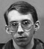
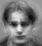
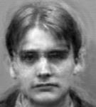
EigenFace Example
➩ EigenFaces are principal components of face images.
➩ Since principal components have the same dimensions as the original items, EigenFaces are images with the same dimensions as the original face images.
➩ Eigenfaces example:
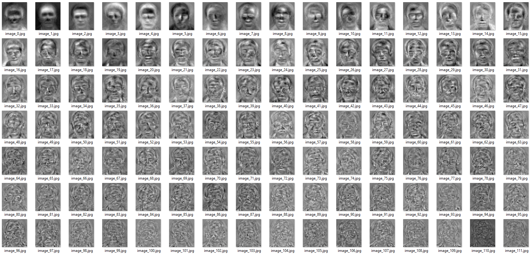
Link
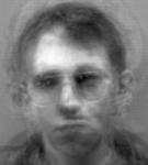
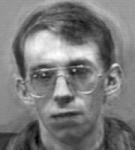
➩ Reconstruction examples:
| K | 1 | 20 | 40 | 50 | 80 |
| Face 1 | 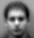
|
|
|

|
|
| Face 2 | 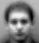
|
|
|

|
|
Images by wellecks
Number of Reduced Dimensions
➩ Similar to other clustering methods, the number of dimensions \(K\) are usually chosen based on application requirements (for example, 2 or 3 for visualization).
➩
sklearn.decomposition.PCA(k) can take in k values between 0 and 1 too, and in that case, k represents the target amount of variance that needs to be explained. 📗 Non-linear PCA
➩ If the kernel trick is used to create new features for PCA, then PCA features are non-linear in the original features, and it's called kernel PCA.
sklearn.decomposition.KernelPCA computes the kernel PCA: Doc. 📗 Auto-Encoder
➩ If a neural network is trained with \(y = x\), then the hidden layer unit values can be viewed as "encoding" of \(x\).
➩ Auto-encoder is a non-linear dimensionality reduction method if the neural network has nonlinear activations.
Additional Examples
➩ Suppose the
explained_variance_ratio of a PCA model is [0.4, 0.3, 0.2, 0.1]. How many components (at least) are needed to explain 80 percent (or more) of the variance of the original data? ➩ 1 component can explain 40 percent.
➩ 2 components can explain 40 + 30 = 70 percent.
➩ 3 components can explain 40 + 30 + 20 = 90 percent, which is more than 80.
➩ At least 3 components are need.
Notes and code adapted from the course taught by Yiyin Shen Link and Tyler Caraza-Harter Link
Last Updated: June 27, 2026 at 9:06 PM