Prev: W14, Next: W15
Zoom: Link, TopHat: Link (936525), GoogleForm: Link, Piazza: Link, Feedback: Link, GitHub: Link, Sec1&2: Link
Slide:
# Dimensionality Reduction
📗 Dimensionality reduction finds a low dimensional representation of a high dimensional point (item) in a way that points that close to each other in the original space are close to each other in the low dimensional space.
➩ Text and image data have a large number of features (dimensions), dimensionality reduction techniques can be used for visualization and efficient storage of these data types: Link.
# Principal Component Analysis
📗 Principal component analysis finds the orthogonal directions that capture the highest variation, called principal components, and project the feature vectors onto the subspace generated by the principal components: Link.
# Projection
📗 A unit vector \(u\) in the direction of a vector \(v\) is \(u = \dfrac{v}{\left\|v\right\|}\), where \(\left\|v\right\| = \sqrt{v_{1}^{2} + v_{2}^{2} + ... v_{m}^{2}}\). Every unit vector satisfy \(u^\top u = 1\).
➩ The projection of a feature vector \(x\) onto the direction of a unit vector \(u\) is \(u^\top x\).
➩ Geometrically, the projection of \(x\) onto \(u\) finds the vector in the direction of \(u\) that is the closest to \(x\).
# Projected Variances
📗 Projected variance along a direction \(u\) is can be computed by \(u^\top \Sigma u\), so the PCA problem is given by the constrained optimization problem \(\displaystyle\max_{u} u^\top \Sigma u\) subject to \(u^\top u = 1\).
➩ A closed-form solution is \(\Sigma u = \lambda u\), which means \(\lambda\) is an eigenvalue of \(\Sigma\) and \(u\) is an eigenvector of \(\Sigma\).
➩ A faster way to find the eigenvalue-eigenvector pair is through singular value decomposition (SVD), and it is used in
sklearn.decomposition.PCA: Doc. US States Economics Data Again, Again
➩ Reduce the dimension of the US states economic data set:
➩ Start with 15 features and find the number of PCA dimensions that can explain 99 percent of the variance.
# Reconstruction
📗 If there are \(m\) original features, and \(m\) principal components are computed, then the original item can be perfectly reconstructed, if only \(k < m\) principal components are used, then the original item can be approximated.
| Feature | Length | Formula | Note |
| Original | \(m\) | \(x = \begin{bmatrix} x_{i 1} \\ x_{i 2} \\ ... \\ x_{i m} \end{bmatrix}\) | - |
| PCA Features | \(k\) | \(x' = \begin{bmatrix} u^\top_{1} x \\ u^\top_{2} x \\ ... \\ u^\top_{k} x \end{bmatrix}\) | \(u_{1}, u_{2}, ...\) are principal components |
| Reconstruction | \(m\) | \(x = x'_{1} u_{1} + x'_{2} u_{2} + ... + x'_{m} u_{m}\) | Equal to original \(x\) |
| Approximation | \(m\) | \(\hat{x} = x'_{1} u_{1} + x'_{2} u_{2} + ... + x'_{k} u_{k} \approx x\) | Length \(m\), not \(k\) |
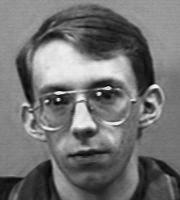
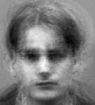
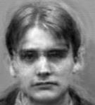
EigenFace Example
➩ EigenFaces are principal components of face images.
➩ Since principal components have the same dimensions as the original items, EigenFaces are images with the same dimensions as the original face images.
➩ Eigenfaces example:
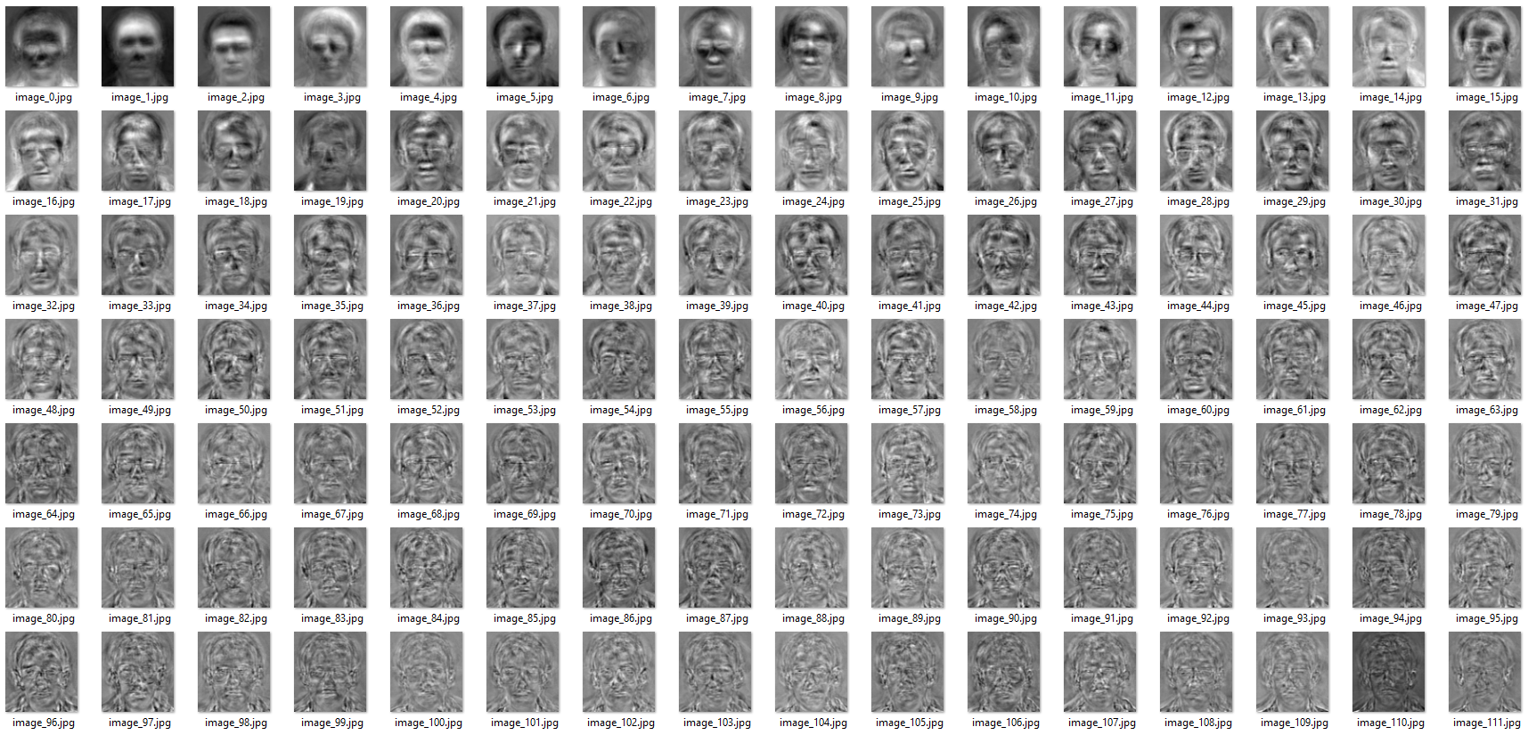
Link
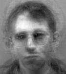
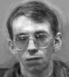
➩ Reconstruction examples:
| K | 1 | 20 | 40 | 50 | 80 |
| Face 1 | 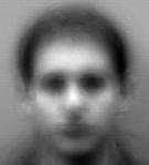
|
|
|

|
|
| Face 2 | 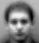
|
|
|

|

|
Images by wellecks
# Number of Reduced Dimensions
📗 Similar to other clustering methods, the number of dimensions \(K\) are usually chosen based on application requirements (for example, 2 or 3 for visualization).
➩
sklearn.decomposition.PCA(k) can take in k values between 0 and 1 too, and in that case, k represents the target amount of variance that needs to be explained. # Non-linear PCA
📗 If the kernel trick is used to create new features for PCA, then PCA features are non-linear in the original features, and it's called kernel PCA.
sklearn.decomposition.KernelPCA computes the kernel PCA: Doc. # Auto-Encoder
📗 If a neural network is trained with \(y = x\), then the hidden layer unit values can be viewed as "encoding" of \(x\).
➩ Auto-encoder is a non-linear dimensionality reduction method if the neural network has nonlinear activations.
# Pseudorandom Numbers
📗 A random sequence can be generated by a recurrence relation, for example, \(x_{t+1} = \left(a x_{t} + c\right) \mod m\).
➩ \(x_{0}\) is called the seed, and if \(a, c, m\) are large and unknown, then the sequence looks random.
➩
numpy.random uses a more complicated PCG generator, but with a similar deterministic sequence that looks random: Link TopHat Discussion
➩ Suppose there are 20 candidates competing for one position, and after interviewing each candidate, the employer has to decide whether to hire the candidate and reject the candidate (cannot hire the rejected candidates later).
➩ The employer's strategy is to interview and reject the first n candidates and hire the first candidate that is better than all n candidates (or the last candidate if none are better).
➩ What is the optimal n?
➩ The problem is called the secretary problem or the marriage problem (date n people and marry the first person that is better than all n): Link
# Questions?
test q
📗 Notes and code adapted from the course taught by Professors Gurmail Singh, Yiyin Shen, Tyler Caraza-Harter.
📗 If there is an issue with TopHat during the lectures, please submit your answers on paper (include your Wisc ID and answers) or this Google form Link at the end of the lecture.
📗 Anonymous feedback can be submitted to: Form. Non-anonymous feedback and questions can be posted on Piazza: Link
Prev: W14, Next: W15
Last Updated: April 06, 2026 at 10:37 PM