Prev: L5, Next: L7 , Assignment: A5 , Practice Questions: M18 M12 M13 , Links: Canvas, Piazza, Zoom, TopHat (453473)
Tools
📗 Calculator:
📗 Canvas:
pen
📗 You can expand all TopHat Quizzes and Discussions: , and print the notes: , or download all text areas as text file: .
# Multi-Layer Perceptron
📗 A single perceptron (with possibly non-linear activation function) still produces a linear decision boundary (the two classes are separated by a line).
📗 Multiple perceptrons can be combined in a way that the output of one perceptron is the input of another perceptron:
➩ \(a^{\left(1\right)} = g\left(w^{\left(1\right)} x + b^{\left(1\right)}\right)\),
➩ \(a^{\left(2\right)} = g\left(w^{\left(2\right)} a^{\left(1\right)} + b^{\left(2\right)}\right)\),
➩ \(a^{\left(3\right)} = g\left(w^{\left(3\right)} a^{\left(2\right)} + b^{\left(3\right)}\right)\),
➩ \(\hat{y} = 1\) if \(a^{\left(3\right)} \geq 0\).
# Neural Networks
➩ Human brain: 100,000,000,000 neurons, each neuron receives input from 1,000 other neurons.
➩ An impulse can either increases or decrease the probability of nerve pulse firing (activation of neuron).
📗 Universal Approximation Theorem: Wikipedia.
➩ A 2-layer network (1 hidden layer) can approximate any continuous function arbitrarily closely with enough hidden units.
➩ A 3-layer network (2 hidden layers) can approximate any function arbitrarily closely with enough hidden units.
In-class Discussion
📗 Try different combinations of activation function and network architecture (number of layers and units in each layer), and compare which ones are good for the spiral dataset: Link.
# Fully Connected Network
📗 The perceptrons will be organized in layers: \(l = 1, 2, ..., L\) and \(m^{\left(l\right)}\) units will be used in layer \(l\).
➩ \(w_{j k}^{\left(l\right)}\) is the weight from unit \(j\) in layer \(l - 1\) to unit \(k\) in layer \(l\), and in the output layer, there is only one unit, so the weights are \(w_{j}^{\left(L\right)}\).
➩ \(b_{j}^{\left(l\right)}\) is the bias for unit \(j\) in layer \(l\), and in the output layer, there is only one unit, so the bias is \(b^{\left(L\right)}\).
➩ \(a_{i j}^{\left(l\right)}\) is the activation for training item \(i\) unit \(j\) in layer \(l\), where \(a_{i j}^{\left(0\right)} = x_{i j}\) can be viewed as unit \(j\) in layer \(0\) (alternatively, \(a_{i j}^{\left(l\right)}\) can be viewed as internal features), and \(a_{i}^{\left(L\right)}\) is the output representing the predicted probability that \(x_{i}\) belongs to class \(1\) or \(\mathbb{P}\left\{\hat{y}_{i} = 1\right\}\).
📗 The way the hidden (internal) units are connected is called the architecture of the network.
📗 In a fully connected network, all units in layer \(l\) are connected to every unit in layer \(l - 1\).
➩ \(a_{i j}^{\left(l\right)} = g\left(a_{i 1}^{\left(l - 1\right)} w_{1 j}^{\left(l\right)} + a_{i 2}^{\left(l - 1\right)} w_{2 j}^{\left(l\right)} + ... + a_{i m^{\left(l - 1\right)}}^{\left(l - 1\right)} w_{m^{\left(l - 1\right)} j}^{\left(l\right)} + b_{j}^{\left(l\right)}\right)\).
Example
📗 [1 points] The following is a diagram of a neural network: highlight an edge (mouse or touch drag from one node to another node) to see the name of the weight (highlight the same edge to hide the name). Highlight color: .
Name of input units: 4
Name of hidden layer 1 units: 3
Name of hidden layer 2 units: 2
Name of hidden layer 3 units: 0
Name of output units: 1
1 slider
In-class Quiz
ID:📗 [4 points] Given the following neural network that classifies all the training instances correctly. What are the labels (0 or 1) of the training data? The activation functions are LTU for all units: \(1_{\left\{z \geq 0\right\}}\). The first layer weight matrix is , with bias vector , and the second layer weight vector is , with bias
| \(x_{i1}\) | \(x_{i2}\) | \(y_{i}\) or \(a^{\left(2\right)}_{1}\) |
| 0 | 0 | ? |
| 0 | 1 | ? |
| 1 | 0 | ? |
| 1 | 1 | ? |
Note: if the weights are not shown clearly, you could move the nodes around with mouse or touch.
📗 Answer (comma separated vector): .
# Gradient Descent
📗 Gradient descent will be used, and the gradient will be computed using chain rule. The algorithm is called backpropogation: Wikipedia.
📗 For a neural network with one input layer, one hidden layer, and one output layer:
➩ \(\dfrac{\partial C_{i}}{\partial w_{j}^{\left(2\right)}} = \dfrac{\partial C_{i}}{\partial a_{i}^{\left(2\right)}} \dfrac{\partial a_{i}^{\left(2\right)}}{\partial w_{j}^{\left(2\right)}}\), for \(j = 1, 2, ..., m^{\left(1\right)}\).
➩ \(\dfrac{\partial C_{i}}{\partial b^{\left(2\right)}} = \dfrac{\partial C_{i}}{\partial a_{i}^{\left(2\right)}} \dfrac{\partial a_{i}^{\left(2\right)}}{\partial b^{\left(2\right)}}\).
➩ \(\dfrac{\partial C_{i}}{\partial w_{j' j}^{\left(1\right)}} = \dfrac{\partial C_{i}}{\partial a_{i}^{\left(2\right)}} \dfrac{\partial a_{i}^{\left(2\right)}}{\partial a_{ij}^{\left(1\right)}} \dfrac{\partial a_{ij}^{\left(1\right)}}{\partial w_{j' j}^{\left(1\right)}}\), for \(j' = 1, 2, ..., m, j = 1, 2, ..., m^{\left(1\right)}\).
➩ \(\dfrac{\partial C_{i}}{\partial b_{j}^{\left(1\right)}} = \dfrac{\partial C_{i}}{\partial a_{i}^{\left(2\right)}} \dfrac{\partial a_{i}^{\left(2\right)}}{\partial a_{ij}^{\left(1\right)}} \dfrac{\partial a_{ij}^{\left(1\right)}}{\partial b_{j}^{\left(1\right)}}\), for \(j = 1, 2, ..., m^{\left(1\right)}\).
📗 More generally, the derivatives can be computed recursively.
➩ \(\dfrac{\partial C_{i}}{\partial b_{j}^{\left(l\right)}} = \left(\dfrac{\partial C_{i}}{\partial b_{1}^{\left(l + 1\right)}} w_{j 1}^{\left(l+1\right)} + \dfrac{\partial C_{i}}{\partial b_{2}^{\left(l + 1\right)}} w_{j 2}^{\left(l+1\right)} + ... + \dfrac{\partial C_{i}}{\partial b_{m^{\left(l + 1\right)}}^{\left(l + 1\right)}} w_{j m^{\left(l + 1\right)}}^{\left(l+1\right)}\right) g'\left(a^{\left(l\right)}_{i j}\right)\), where \(\dfrac{\partial C_{i}}{\partial b^{\left(L\right)}} = \dfrac{\partial C_{i}}{\partial a_{i}^{\left(L\right)}} g'\left(a_{i}^{\left(L\right)}\right)\).
➩ \(\dfrac{\partial C_{i}}{\partial w_{j' j}^{\left(l\right)}} = \dfrac{\partial C_{i}}{\partial b_{j}^{\left(l\right)}} a_{i j'}^{\left(l - 1\right)}\).
📗 Gradient descent formula is the same: \(w = w - \alpha \left(\nabla_{w} C_{1} + \nabla_{w} C_{2} + ... + \nabla_{w} C_{n}\right)\) and \(b = b - \alpha \left(\nabla_{b} C_{1} + \nabla_{b} C_{2} + ... + \nabla_{b} C_{n}\right)\) for all the weights and biases.
Example
📗 PyTorch code example: Link.
📗 For two layer neural network with sigmoid activations (used in logistic regression) and square loss,
➩ The
\(a^{\left(1\right)}_{ij} = \dfrac{1}{1 + \exp\left(- \left(\left(\displaystyle\sum_{j'=1}^{m} x_{ij'} w^{\left(1\right)}_{j'j}\right) + b^{\left(1\right)}_{j}\right)\right)}\) for j = 1, ..., h, forward() step in PyTorch: \(a^{\left(2\right)}_{i} = \dfrac{1}{1 + \exp\left(- \left(\left(\displaystyle\sum_{j=1}^{h} a^{\left(1\right)}_{ij} w^{\left(2\right)}_{j}\right) + b^{\left(2\right)}\right)\right)}\),
➩ The
\(\dfrac{\partial C_{i}}{\partial w^{\left(1\right)}_{j'j}} = \left(a^{\left(2\right)}_{i} - y_{i}\right) a^{\left(2\right)}_{i} \left(1 - a^{\left(2\right)}_{i}\right) w_{j}^{\left(2\right)} a_{ij}^{\left(1\right)} \left(1 - a_{ij}^{\left(1\right)}\right) x_{ij'}\) for j' = 1, ..., m, j = 1, ..., h, backward() step in PyTorch: \(\dfrac{\partial C_{i}}{\partial b^{\left(1\right)}_{j}} = \left(a^{\left(2\right)}_{i} - y_{i}\right) a^{\left(2\right)}_{i} \left(1 - a^{\left(2\right)}_{i}\right) w_{j}^{\left(2\right)} a_{ij}^{\left(1\right)} \left(1 - a_{ij}^{\left(1\right)}\right)\) for j = 1, ..., h,
\(\dfrac{\partial C_{i}}{\partial w^{\left(2\right)}_{j}} = \left(a^{\left(2\right)}_{i} - y_{i}\right) a^{\left(2\right)}_{i} \left(1 - a^{\left(2\right)}_{i}\right) a_{ij}^{\left(1\right)}\) for j = 1, ..., h,
\(\dfrac{\partial C_{i}}{\partial b^{\left(2\right)}} = \left(a^{\left(2\right)}_{i} - y_{i}\right) a^{\left(2\right)}_{i} \left(1 - a^{\left(2\right)}_{i}\right)\),
\(w^{\left(1\right)}_{j' j} \leftarrow w^{\left(1\right)}_{j' j} - \alpha \dfrac{\partial C_{i}}{\partial w^{\left(1\right)}_{j' j}}\) for j' = 1, ..., m, j = 1, ..., h,
\(b^{\left(1\right)}_{j} \leftarrow b^{\left(1\right)}_{j} - \alpha \dfrac{\partial C_{i}}{\partial b^{\left(1\right)}_{j}}\) for j = 1, ..., h,
\(w^{\left(2\right)}_{j} \leftarrow w^{\left(2\right)}_{j} - \alpha \dfrac{\partial C_{i}}{\partial w^{\left(2\right)}_{j}}\) for j = 1, ..., h,
\(b^{\left(2\right)} \leftarrow b^{\left(2\right)} - \alpha \dfrac{\partial C_{i}}{\partial b^{\left(2\right)}}\).
In-class Quiz
📗 Highlight the weights used in computing \(\dfrac{\partial C}{\partial w^{\left(1\right)}_{11}}\) in the backpropogation step.
📗 [1 points] The following is a diagram of a neural network: highlight an edge (mouse or touch drag from one node to another node) to see the name of the weight (highlight the same edge to hide the name). Highlight color: .
Name of input units: 4
Name of hidden layer 1 units: 3
Name of hidden layer 2 units: 2
Name of hidden layer 3 units: 0
Name of output units: 1
1 slider
# Stochastic Gradient Descent
📗 The gradient descent algorithm updates the weight using the gradient which is the sum over all items, for logistic regression: \(w = w - \alpha \left(\left(a_{1} - y_{1}\right) x_{1} + \left(a_{2} - y_{2}\right) x_{2} + ... + \left(a_{n} - y_{n}\right) x_{n}\right)\).
📗 A variant of the gradient descent algorithm that updates the weight for one item at a time is called stochastic gradient descent. This is because the expected value of \(\dfrac{\partial C_{i}}{\partial w}\) for a random \(i\) is equal to \(\dfrac{\partial C}{\partial w}\): Wikipedia.
➩ Gradient descent (batch): \(w = w - \alpha \dfrac{\partial C}{\partial w}\) or \(w = w - \alpha \left(\dfrac{\partial C_{1}}{\partial w} + \dfrac{\partial C_{2}}{\partial w} + ... + \dfrac{\partial C_{n}}{\partial w}\right)\).
➩ Stochastic gradient descent: for a random \(i \in \left\{1, 2, ..., n\right\}\), \(w = w - \alpha \dfrac{\partial C_{i}}{\partial w}\).
📗 Instead of randomly pick one item at a time, the training set is usually shuffled, and the shuffled items will be used to update the weights and biases in order. Looping through all items once is called an epoch.
➩ Stochastic gradient descent can also help moving out of a local minimum of the cost function: Link.
Example
📗 [1 points] Suppose the minimum occurs at the center of the plot: the following are paths based on (batch) gradient descent [red] vs stochastic gradient descent [blue]. Move the green point to change the starting point.
Math Note
📗 Note: the Perceptron algorithm updates the weight for one item at a time: \(w = w - \alpha \left(a_{i} - y_{i}\right) x_{i}\), but it is not gradient descent or stochastic gradient descent.
# Softmax Layer
📗 For both logistic regression and neural network, the output layer can have \(K\) units, \(a_{i k}^{\left(L\right)}\), for \(k = 1, 2, ..., K\), for K-class classification problems: Link,
📗 The labels should be converted to one-hot encoding, \(y_{i k} = 1\) when the true label is \(k\) and \(y_{i k} = 0\) otherwise.
➩ If there are \(K = 3\) classes, then all items with true label \(1\) should be converted to \(y_{i} = \begin{bmatrix} 1 \\ 0 \\ 0 \end{bmatrix}\), and true label \(2\) to \(y_{i} = \begin{bmatrix} 0 \\ 1 \\ 0 \end{bmatrix}\), and true label \(3\) to \(y_{i} = \begin{bmatrix} 0 \\ 0 \\ 1 \end{bmatrix}\).
📗 The last layer should normalize the sum of all \(K\) units to \(1\). A popular choice is the softmax operation: \(a_{i k}^{\left(L\right)} = \dfrac{e^{z_{i k}}}{e^{z_{i 1}} + e^{z_{i 2}} + ... + e^{z_{i K}}}\), where \(z_{i k} = w_{1 k} a_{i 1}^{\left(L - 1\right)} + w_{2 k} a_{i 2}^{\left(L - 1\right)} + ... w_{m^{\left(L - 1\right)} k} a_{i m^{\left(L - 1\right)}}^{\left(L - 1\right)} + b_{k}\) for \(k = 1, 2, ..., K\): Wikipedia.
Example
📗 [1 points] The following is a diagram of a neural network: highlight an edge (mouse or touch drag from one node to another node) to see the name of the weight (highlight the same edge to hide the name). Highlight color: .
Name of input units: 4
Name of hidden layer 1 units: 3
Name of hidden layer 2 units: 2
Name of hidden layer 3 units: 0
Name of output units: 1
1 slider
Math Note
📗 If cross entropy loss is used, \(C_{i} = -y_{i 1} \log\left(a_{i 1}\right) - y_{i 2} \log\left(a_{i 2}\right) + ... - y_{i K} \log\left(a_{i K}\right)\), then the derivative can be simplified to \(\dfrac{\partial C_{i}}{\partial z_{i k}} = a^{\left(L\right)}_{i k} - y_{i k}\) or \(\nabla_{z_{i}} C_{i} = a^{\left(L\right)}_{i} - y_{i}\).
➩ Some calculus:
\(C_{i} = - \displaystyle\sum_{k=1}^{K} y_{i k} \log \dfrac{e^{z_{i k}}}{\displaystyle\sum_{k' = 1}^{K} e^{z_{i k'}}}\) \(= \displaystyle\sum_{k=1}^{K} y_{i k} \log \left(\displaystyle\sum_{k=1}^{K} e^{z_{i k}}\right) - \displaystyle\sum_{k=1}^{K} y_{i k} z_{i k}\)
\(= \log \left(\displaystyle\sum_{k=1}^{K} e^{z_{i k}}\right) - \displaystyle\sum_{k=1}^{K} y_{i k} z_{i k}\) since \(y_{i k}\) sum up to \(1\) for a fixed item \(i\).
\(\dfrac{\partial C_{i}}{\partial z_{i k}} = \dfrac{e^{z_{i k}}}{\displaystyle\sum_{k' = 1}^{K} e^{z_{i k'}}} - y_{i k} = a^{\left(L\right)}_{i k} - y_{i k}\)
\(\nabla_{z_{i}} C_{i} = a^{\left(L\right)}_{i} - y_{i}\).
# Function Approximator
📗 Neural networks can be used in different areas of machine learning.
➩ In supervised learning, a neural network approximates \(\mathbb{P}\left\{y | x\right\}\) as a function of \(x\).
➩ In unsupervised learning, a neural network can be used to perform non-linear dimensionality reduction. Training a neural network with output \(y_{i} = x_{i}\) and fewer hidden units than input units will find a lower dimensional representation (the values of the hidden units) of the inputs. This is called an auto-encoder: Wikipedia.
➩ In reinforcement learning, there can be multiple neural networks to store and approximate the value function and the optimal policy (choice of actions): Wikipedia.
# Generalization Error
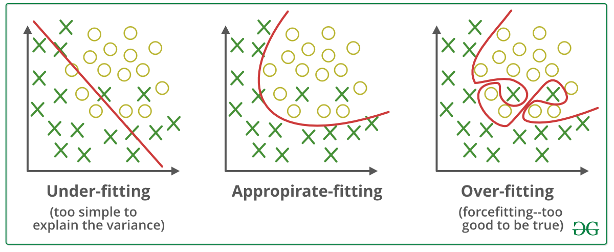
📗 With a large number of hidden layers and units, a neural network can overfit a training set perfectly. This does not imply the performance on new items will be good: Wikipedia.
➩ More data can be created for training using generative models or unsupervised learning techniques.
➩ A validation set can be used (similar to pruning for decision trees) to train the network until the loss (or accuracy) on the validation set begins to increase.
➩ Dropout can be used: randomly omitting units (random pruning of weights) during training so the rest of the units will have a better performance: Wikipedia.
Example
# Regularization
📗 A simpler model (with fewer weights, or many weights set to 0) is usually more generalizable and would not overfit the training set as much. A way to achieve that is to include an additional cost for non-zero weights during training. This is called regularization: Wikipedia.
➩ \(L_{1}\) regularization adds \(L_{1}\) norm of the weights and biases to the loss, or \(C = C_{1} + C_{2} + ... + C_{n} + \lambda \left\|\begin{bmatrix} w \\ b \end{bmatrix}\right\|_{1}\), for example, if there are no hidden layers, \(\left\|\begin{bmatrix} w \\ b \end{bmatrix}\right\|_{1} = \left| w_{1} \right| + \left| w_{2} \right| + ... + \left| w_{m} \right| + \left| b \right|\). Linear regression with \(L_{1}\) regularization is also called LASSO (Least Absolute Shrinkage and Selector Operator): Wikipedia.
➩ \(L_{2}\) regularization adds \(L_{2}\) norm of the weights and biases to the loss, or \(C = C_{1} + C_{2} + ... + C_{n} + \lambda \left\|\begin{bmatrix} w \\ b \end{bmatrix}\right\|^{2}_{2}\), for example, if there are no hidden layers, \(\left\|\begin{bmatrix} w \\ b \end{bmatrix}\right\|^{2}_{2} = \left(w_{1}\right)^{2} + \left(w_{2}\right)^{2} + ... + \left(w_{m}\right)^{2} + \left(b\right)^{2}\). Linear regression with \(L_{2}\) regularization is also called ridge regression: Wikipedia.
📗 \(\lambda\) is chosen as the trade-off between the loss from incorrect prediction and the loss from non-zero weights.
➩ \(L_{1}\) regularization often leads to more weights that are exactly \(0\), which is useful for feature selection.
➩ \(L_{2}\) regularization is easier for gradient descent since it is differentiable.
➩ Try \(L_{1}\) vs \(L_{2}\) regularization here: Link.
In-class Discussion
📗 [1 points] Fix some \(d\), find the point where \(\left\|\begin{bmatrix} w_{1} \\ w_{2} \end{bmatrix}\right\| \leq d\) and minimize the cost \(c\). Use regularization.
➩ Aside: compare the above procedure with: fix some cost \(c\), find the point with the minimum distance to the origin \(d\). This is related to this duality of optimization.
Bound \(d\): 0.5
Cost \(C\): 0
1 slider
# Margin and Support Vectors
📗 The perceptron algorithm finds any one of many linear classifier that separates two classes.
📗 Among them, the classifier with the widest margin (width of the thickest line that can separate the two classes) is call the support vector machine (the items or feature vectors on the edges of the thick line are called support vectors).
In-class Discussion
ID:📗 [1 points] Move the line (by moving the two points on the line) so that it separates the two classes and the margin is maximized.
Margin: 0 1
slider
In-class Discussion
ID:📗 [1 points] Move the plus (blue) and minus (red) planes so that they separate the two classes and the margin is maximized.
Plane: 0
Margin: 0 1
slider
# Hard Margin Support Vector Machine
📗 Mathematically, the margins can be computed by \(\dfrac{2}{\sqrt{w^\top w}}\) or \(\dfrac{2}{\sqrt{w_{1}^{2} + w_{2}^{2} + ... + w_{m}^{2}}}\), which is the distance between the two edges of the thick line (or two hyper-planes in high dimensional space), \(w^\top x_{i} + b = w_{1} x_{i 1} + w_{2} x_{i 2} + ... + w_{m} x_{i m} + b = \pm 1\).
📗 The optimization problem is given by \(\displaystyle\max_{w} \dfrac{2}{\sqrt{w^\top w}}\) subject to \(w^\top x_{i} + b \leq -1\) if \(y_{i} = 0\) and \(w^\top x_{i} + b \geq 1\) if \(y_{i} = 1\) for \(i = 1, 2, ..., n\).
📗 The problem is equivalent to \(\displaystyle\min_{w} \dfrac{1}{2} w^\top w\) subject to \(\left(2 y_{i} - 1\right) \left(w^\top x_{i} + b\right) \geq 1\) for \(i = 1, 2, ..., n\).
# Soft Margin Support Vector Machine
📗 To allow mistakes classifying a few items (similar to logistic regression), slack variables \(\xi_{i}\) can be introduced.
📗 The problem can be modified to \(\displaystyle\min_{w} \dfrac{1}{2} w^\top w + \dfrac{1}{\lambda} \dfrac{1}{n} \left(\xi_{1} + \xi_{2} + ... + \xi_{n}\right)\) subject to \(\left(2 y_{i} - 1\right) \left(w^\top x_{i} + b\right) \geq 1 - \xi_{i}\) and \(\xi_{i} \geq 0\) for \(i = 1, 2, ..., n\).
📗 The problem is equivalent to \(\displaystyle\min_{w} \dfrac{\lambda}{2} w^\top w + \dfrac{1}{n} \left(C_{1} + C_{2} + ... + C_{n}\right)\) where \(C_{i} = \displaystyle\max\left\{0, 1 - \left(2 y_{i} - 1\right)\left(w^\top x_{i} + b\right)\right\}\).
➩ This is similar to \(L_{2}\) regularized perceptrons with hinge loss (which will be introduced in a future lecture).
In-class Discussion
ID:📗 [1 points] Move the line (by moving the two points on the line) so that the regularized loss is minimized: margin = , average slack = , loss = , where \(\lambda\) = .
Margin: 0 1
slider
Other students' answers:
In-class Discussion
ID:📗 [1 points] Move the plus (blue) and minus (red) planes so that the regularized loss is minimized: margin = , average slack = , loss = , where \(\lambda\) = .
Plane: 0
Margin: 0 1
slider
Other students' answers:
# Subgradient Descent
📗 Gradient descent can be used to choose the weights by minimizing the costs, but the hinge loss function is not differentiable at some points. At those points, sub-derivative (or sub-gradient) can be used instead.
Math Note
📗 Sub-derivative at a point is the slope of any of the tangent lines at the point.
➩ Define \(y'_{i} = 2 y_{i} - 1\) (convert \(y_{i} = 0, 1\) to \(y'_{i} = -1, 1\), subgradeint descent for soft margin support vector machine is \(w = \left(1 - \lambda\right) w - \alpha \left(C'_{1} + C'_{2} + ... + C'_{n}\right)\) where \(C'_{i} = y'_{i}\) if \(y'_{i} w^\top x_{i} \geq 1\) and \(C'_{i} = 0\) otherwise. \(b\) is usually set to 0 for support vector machines.
➩ Stochastic gradient descent \(w = \left(1 - \lambda\right) w - \alpha C'_{i}\) for \(i = 1, 2, ..., n\) for support vector machines is called PEGASOS (Primal Estimated sub-GrAdient SOlver for Svm).
In-class Quiz
ID:📗 [1 points] What are the smallest and largest values of subderivatives of at \(x = 0\).
📗 Answer:
Min (green line): 0 Max (blue line): 0 1
slider
Other students' answers:
# Multi-Class SVM
📗 Multiple SVMs can be trained to perform multi-class classification.
➩ One-vs-one: \(\dfrac{1}{2} K \left(K - 1\right)\) classifiers (if there are \(K = 3\) classes then the classifiers are 1 vs 2, 1 vs 3, 2 vs 3.
➩ One-vs-all (or one-vs-rest): \(K\) classifiers (if there are \(K = 3\) classes then the classifiers are 1 vs not-1, 2 vs not-2, 3 vs not-3.
# Feature Map
📗 If the classes are not linearly separable, more features can be created so that in the higher dimensional space, the items might be linearly separable. This applies to perceptrons and support vector machines.
📗 Given a feature map \(\varphi\), the new items \(\left(\varphi\left(x_{i}\right), y_{i}\right)\) for \(i = 1, 2, ..., n\) can be used to train perceptrons or support vector machines.
📗 When applying the resulting classifier on a new item \(x_{i'}\), \(\varphi\left(x_{i'}\right)\) should be used as the features too.
In-class Discussion
ID:📗 [1 points] Transform the points (using the feature map) and move the plane such that the plane separates the two classes.
Feature map scale: 0
Plane: 0 0
slider
Other students' answers:
# Kernel Trick
📗 Using non-linear feature maps for support vector machines (which are linear classifiers) is called the kernel trick since any feature map on a data set can be represented by a \(n \times n\) matrix called the kernel matrix (or Gram matrix): \(K_{i i'} = \varphi\left(x_{i}\right)^\top \varphi\left(x_{i'}\right) = \varphi_{1}\left(x_{i}\right) \varphi_{1}\left(x_{i'}\right) + \varphi_{2}\left(x_{i}\right) \varphi_{2}\left(x_{i'}\right) + ... + \varphi_{m}\left(x_{i}\right) \varphi_{m}\left(x_{i'}\right)\), for \(i = 1, 2, ..., n\) and \(i' = 1, 2, ..., n\).
➩ If \(\varphi\left(x_{i}\right) = \begin{bmatrix} x_{i 1}^{2} \\ \sqrt{2} x_{i 1} x_{i 2} \\ x_{i 2}^{2} \end{bmatrix}\), then \(K_{i i'} = \left(x^\top_{i} x_{i'}\right)^{2}\).
➩ If \(\varphi\left(x_{i}\right) = \begin{bmatrix} \sqrt{2} x_{i 1} \\ x_{i 1}^{2} \\ \sqrt{2} x_{i 1} x_{i 2} \\ x_{i 2}^{2} \\ \sqrt{2} x_{i 2} \\ 1 \end{bmatrix}\), then \(K_{i i'} = \left(x^\top_{i} x_{i'} + 1\right)^{2}\).
In-class Quiz
ID:📗 [4 points] Consider a kernel \(K\left(x_{i_{1}}, x_{i_{2}}\right)\) = + + , where both \(x_{i_{1}}\) and \(x_{i_{2}}\) are 1D positive real numbers. What is the feature vector \(\varphi\left(x_{i}\right)\) induced by this kernel evaluated at \(x_{i}\) = ?
📗 Answer (comma separated vector): .
# Kernel Matrix
📗 A matrix is a kernel for some feature map \(\varphi\) if and only if it is symmetric positive semi-definite (positive semi-definiteness is equivalent to having non-negative eigenvalues).
📗 Some kernel matrices correspond to infinite-dimensional feature maps.
➩ Linear kernel: \(K_{i i'} = x^\top_{i} x_{i'}\).
➩ Polynomial kernel: \(K_{i i'} = \left(x^\top_{i} x_{i'} + 1\right)^{d}\).
➩ Radial basis function (Gaussian) kernel: \(K_{i i'} = e^{- \dfrac{1}{\sigma^{2}} \left(x_{i} - x_{i'}\right)^\top \left(x_{i} - x_{i'}\right)}\). In this case, the new features are infinite dimensional (any finite data set is linearly separable), and dual optimization techniques are used to find the weights (subgradient descent for the primal problem cannot be used).
Math Note
➩ The primal problem is given by \(\displaystyle\min_{w} \dfrac{\lambda}{2} w^\top w + \dfrac{1}{n} \displaystyle\sum_{i=1}^{n} \displaystyle\max\left\{0, 1 - \left(2 y_{i} - 1\right) \left(w^\top x_{i} + b\right)\right\}\),
➩ The dual problem is given by \(\displaystyle\max_{\alpha > 0} \displaystyle\sum_{i=1}^{n} \alpha_{i} - \dfrac{1}{2} \displaystyle\sum_{i,i' = 1}^{n} \alpha_{i} \alpha_{i'} \left(2 y_{i} - 1\right) \left(2 y_{i'} - 1\right) \left(x^\top_{i} x_{i'}\right)\) subject to \(0 \leq \alpha_{i} \leq \dfrac{1}{\lambda n}\) and \(\displaystyle\sum_{i=1}^{n} \alpha_{i} \left(2 y_{i} - 1\right) = 0\).
➩ The dual problem only involves \(x^\top_{i} x_{i'}\), and with the new features, \(\varphi\left(x_{i}\right)^\top \varphi\left(x_{i'}\right)\) which are elements of the kernel matrix.
➩ The primal classifier is \(w^\top x + b\).
➩ The dual classifier is \(\displaystyle\sum_{i=1}^{n} \alpha_{i} y_{i} \left(x^\top_{i} x\right) + b\), where \(\alpha_{i} \neq 0\) only when \(x_{i}\) is a support vector.
test nnd,ann,sgd,sfm,rd,sd,st,sf,ss,sg,kt,fv q
📗 Notes and code adapted from the course taught by Professors Jerry Zhu, Yingyu Liang, and Charles Dyer.
📗 Please use Ctrl+F5 or Shift+F5 or Shift+Command+R or Incognito mode or Private Browsing to refresh the cached JavaScript.
📗 Anonymous feedback can be submitted to: Form.
Prev: L5, Next: L7
Last Updated: June 27, 2026 at 9:07 PM