Prev: W12, Next: W14
Zoom: Link, TopHat: Link (341925), GoogleForm: Link, Piazza: Link, Feedback: Link.
Slide:
# Deep Q Learning
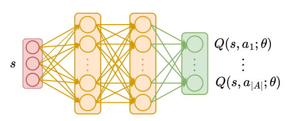
📗 In practice, Q function stored as a table is too large if the number of states is large or infinite (the action space is usually finite): Link, Link, Wikipedia.
📗 If there are \(m\) binary features that represent the state, then the Q table contains \(2^{m} \left| A \right|\), which can be intractable.
📗 In this case, a neural network can be used to store the Q function, and if there is a single layer with \(m\) units, then only \(m^{2} + m \left| A \right|\) weights are needed.
➩ The input of the network \(\hat{Q}\) is the features of the state \(s\), and the outputs of the network are Q values associated with the actions \(a\) or \(Q\left(s, a\right)\) (the output layer does not need to be softmax since the Q values for different actions do not need to sum up to \(1\)).
➩ After every iteration, the network can be updated based on an item \(\left(s_{t}, \left(1 - \alpha\right) \hat{Q}\left(s_{t}, a_{t}\right) + \alpha \left(r_{t} + \beta \displaystyle\max_{a} \hat{Q}\left(s_{t+1}, a\right)\right)\right)\).
# Deep Q Network
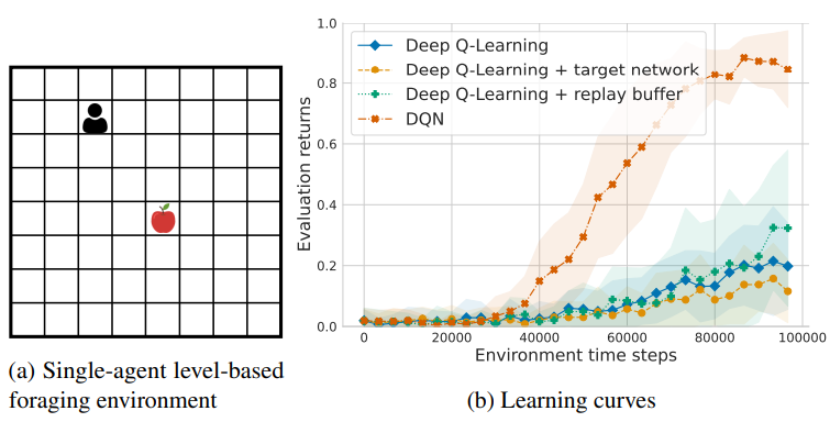
📗 Deep Q Learning algorithm is unstable since the training label uses the network itself. The following improvements can be made to make the algorithm more stable, called DQN (Deep Q Network).
➩ Target network: two networks can be used, the Q network \(\hat{Q}\) and the target network \(Q'\), and the new item for training \(\hat{Q}\) can be changed to \(\left(s_{t}, \left(1 - \alpha\right) Q'\left(s_{t}, a_{t}\right) + \alpha \left(r_{t} + \beta \displaystyle\max_{a} Q'\left(s_{t+1}, a\right)\right)\right)\).
➩ Experience replay: some training data can be saved and a mini-batch (sampled from the training set) can be used to update \(\hat{Q}\) instead of a single item.
Example
# Policy Gradient
📗 Deep Q Network estimates the Q function as a neural network, and the policy can be computed as \(\pi\left(s\right) = \mathop{\mathrm{argmax}}_{a} \hat{Q}\left(s, a\right)\), which is always deterministic.
➩ In single-agent reinforcement learning, there is always a deterministic optimal policy, so DQN can be used to solve for an optimal policy.
➩ In multi-agent reinforcement learning, the optimal equilibrium policy can be all stochastic (mixed strategy equilibrium): Wikipedia.
📗 The policy can also be represented by a neural network called the policy network \(\hat{\pi}\) and it can be trained with or without using a value network \(\hat{V}\).
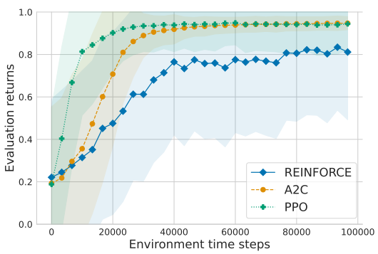
➩ Without a value network: REINFORCE (REward Increment = Non-negative Factor x Offset x Characteristic Eligibility).
➩ With a value network: A2C (Advantage Actor Critic) and PPO (Proximal Policy Optimization).
📗 To train the policy network \(\hat{\pi}\), the input is the features of the state \(s\) and the output units (softmax output layer) are the probability of using each action \(a\) or \(\mathbb{P}\left\{\pi\left(s\right) = a\right\}\). The cost function the network minimizes can be value function (REINFORCE) or the advantage function (difference between value and Q, A2C and PPO).
📗 The value network is trained in a way similar to DQN.
Example
Math Note (Optional)
📗 Policy gradient theorem: \(\nabla_{w} V\left(w\right) = \mathbb{E}\left[Q^{\hat{\pi}}\left(s, a\right) \nabla_{w} \log \hat{\pi}\left(a | s; w\right)\right]\)
➩ Given this gradient formula, the loss for the policy network in REINFORCE can be written as \(\left(\displaystyle\sum_{t'=t+1}^{T} \beta^{t'-t-1} r_{t'}\right) \log \pi\left(a_{t} | s_{t} ; w\right)\), where \(\displaystyle\sum_{t'=t+1}^{T} \beta^{t'-t-1} r_{t'}\) is an estimate of \(Q^{\hat{\pi}}\left(s_{t}, a_{t}\right)\).
➩ The loss for the policy network in A2C is \(-\left(r_{t} + \beta \hat{V}\left(s_{t+1}\right) - \hat{V}\left(s_{t}\right)\right) \log \pi\left(a_{t} | s_{t} ; w\right)\), where \(r_{t} + \beta \hat{V}\left(s_{t+1}\right) - \hat{V}\left(s_{t}\right)\) is an estimate of the advantage function \(Q^{\hat{\pi}}\left(s_{t}, a_{t}\right) - V^{\hat{\pi}}\left(s_{t}\right)\).
# Multi-Agent Reinforcement Learning
📗 Multi-Agent Reinforcement Learning (MARL) is harder than Single Agent RL.
| Single Agent RL | Multi Agent RL |
| MDP stationary | Non-stationary environment |
| Unique optimal value | Multiple equilibria with different values |
| One Agent | Problem scales exponentially with number of agents |
# Markov Game
📗 Full observation MARL problems are modeled by Markov Games (MGs, or Stochastic Games): \((I, S, A, R, P)\).
➩ \(I\) is the set of players.
➩ \(S\) is the set of states (common to all players).
➩ \(A = \displaystyle\prod_{i \in I} A_{i}\) is the set of actions.
➩ \(R_{i} : S \times A \to \mathbb{R}\) is the reward function for player \(i \in I\).
➩ \(P : S \times A \to \Delta S\) is the state transition function (common to all players).
➩ \(P\left(\emptyset\right) \in \Delta S\) is the initial state distribution.
# Reduction to Single Agent RL
📗 Centralized Q-Learning: define joint reward (sometimes called social welfare function) and treat \(a \in A = \displaystyle\prod_{i \in I} A_{i}\) as the action space.
📗 Indepedent Q-Learning: single agent RL algorithm to control each agent, often does not converge.
# Value Iteration
📗 Value iteration for MGs, repeat until converge:
➩ \(Q_{i}\left(s, a\right) = R_{i}\left(s, a\right) + \beta \displaystyle\sum_{s' \in S} P\left(s' | s, a\right) V_{i}\left(s'\right)\).
➩ \(V_{i}\left(s\right) = \text{NE}\left(Q\left(s, \cdot\right)\right)\), where Nash Equilibrium (NE) can be replaced by other game equilibrium concepts (for example Correlated Equilibrium (CE) or Coarse Correlated Equilibrium (CCE)).
📗 The solution (Nash equilibrium policy, if converges) is called Markov Perfect Equilibrium (MPE).
📗 Learning, with for example, epsilon-Greedy:
➩ With probably \(\varepsilon\), choose a random action, otherwise, sample \(a_{t} \sim \pi\left(s_{t}\right) \in \text{NE}\left(Q\left(s_{t}, \cdot\right)\right)\), and observe reward \(r_{t}, s_{t+1}\).
➩ Update \(Q\left(s_{t}, a_{t}\right) = Q\left(s_{t}, a_{t}\right) + \alpha \left(r_{t} + \beta \text{NE}\left(Q\left(s_{t+1}, \cdot\right)\right) - Q\left(s_{t}, a_{t}\right)\right)\).
# Minimax Q-Learning
📗 \(\text{NE}\left(Q\left(s, \cdot\right)\right)\) is not unique for general-sum games, meaning for general-sum MGs, value functions are not defined.
📗 \(\text{NE}\left(Q\left(s, \cdot\right)\right)\) is unique for zero-sum games, minimax-Q (use minimax solver for stage game \(Q\left(s, \cdot\right)\)) converges to an MPE.
Soccer Game Example
📗 Grid-world soccer game (numbers are percentage won and episode length)
| - | minimax Q | independent Q |
| vs random | \(99.3 \left(13.89\right)\) | \(99.5 \left(11.63\right)\) |
| vs hand-built | \(53.7 \left(18.87\right)\) | \(76.3 \left(30.30\right)\) |
| vs optimal | \(37.5 \left(22.73\right)\) | \(0 \left(83.33\right)\) |

(Littman 1994: PDF)
# Nash Q-Learning
📗 Equilibrium selection by finding the Nash equilibrium with the highest sum of rewards (computationally intractable).
📗 Nash Q is guaranteed to converge under very restrictive assumptions.
➩ CE or CCE can be used in place of NE (CE and CCE can be solved with a linear program, easier than NE).
➩ No known condition for Correlated Q to converge.
# Deep MARL
📗 Most of the deep MARL models assume partial observability (recurrent units or attention modules) and uses either centralized or independent learning (through best response dynamics, similar to GAN).
➩ Hide and seek: Link.
➩ Adversarial attack on one player: Link.
➩ UW Madison Soccer Team: Link.
test q
📗 Notes and code adapted from the course taught by Professors Blerina Gkotse, Jerry Zhu, Yudong Chen, Yingyu Liang, Charles Dyer.
📗 If there is an issue with TopHat during the lectures, please submit your answers on paper (include your Wisc ID and answers) or this Google form Link at the end of the lecture.
📗 Anonymous feedback can be submitted to: Form. Non-anonymous feedback and questions can be posted on Piazza: Link
Prev: W12, Next: W14
Last Updated: June 27, 2026 at 9:07 PM