Prev: W4 Next: W6
Blank Slides (with blank pages for quiz questions): Part 1, Part 2,
Annotated Slides: Part 1, Part 2,

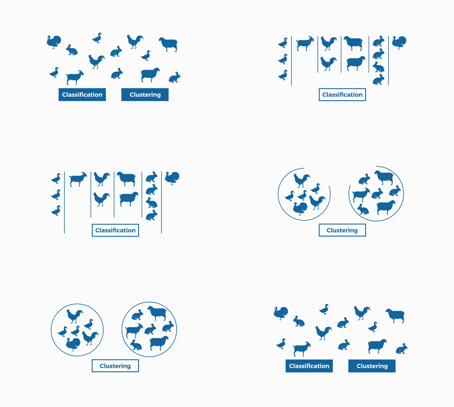
Image by bismart
Lecture 15 Part 2 (Hierarchical Clustering): Link
Lecture 15 Part 3 (K Means Clustering): Link
Lecture 16 Part 1 (Dimensionality Reduction): Link
Lecture 16 Part 2 (Principal Component): Link
Lecture 16 Part 3 (Non-linear PCA): Link
Hierachical Clustering: Link
Tree of Life: Link 1, Link 2
K Means Clustering: Link
K Gaussian Mixture: Link
Word Embedding: Link
Principal Component: Link
Eigen Face: Link 1, Link 2
t-distributed Stochastic Neighbor Embedding: Link
tSNE Demo: Link
Swiss Roll: Link
PCA Proofs from Professor Jerry Zhu's 540 notes: PDF File
How to compute optimal value function? Link
What is the relationship between Naive Bayes and Logistic Regression? Link
What is the relationship between K Means and Gradient Descent? Link
Why is PCA solving eigenvalues and eigenvectors? Part 1, Part 2, Part 3
How to update distance table for hierarchical clustering? Link
How to update cluster centers for K-means clustering? Link
How to compute projection? Link
How to compute new features based on PCA? Link
# Summary
📗 Tuesday to Friday lectures: 1:00 to 2:15, Zoom Link
📗 Saturday review sessions: 5:30 to 8:30, Zoom Link
📗 Personal meeting room: always open, Zoom Link
📗 Quiz (use your wisc ID to log in (without "@wisc.edu")): Socrative Link
📗 Math Homework:
M8,
📗 Programming Homework:
P4,
📗 Examples and Quizzes:
Q15,
Q16,
# Lectures
📗 Slides (before lecture, usually updated on Sunday):
Blank Slides:
Part 1,
Part 2,
Blank Slides (with blank pages for quiz questions): Part 1, Part 2,
📗 Slides (after lecture, usually updated on Friday):
Blank Slides with Quiz Questions:
Part 1,
Part 2,
Annotated Slides: Part 1, Part 2,
📗 Review Session:
PDF. 📗 My handwriting is really bad, you should copy down your notes from the lecture videos instead of using these.
📗 Notes

Image by bismart
# Other Materials
📗 Pre-recorded Videos from 2020
Lecture 15 Part 1 (Unsupervised Learning): Link Lecture 15 Part 2 (Hierarchical Clustering): Link
Lecture 15 Part 3 (K Means Clustering): Link
Lecture 16 Part 1 (Dimensionality Reduction): Link
Lecture 16 Part 2 (Principal Component): Link
Lecture 16 Part 3 (Non-linear PCA): Link
📗 Relevant websites
Image Segmentation: Link 1, Link 2 Hierachical Clustering: Link
Tree of Life: Link 1, Link 2
K Means Clustering: Link
K Gaussian Mixture: Link
Word Embedding: Link
Principal Component: Link
Eigen Face: Link 1, Link 2
t-distributed Stochastic Neighbor Embedding: Link
tSNE Demo: Link
Swiss Roll: Link
PCA Proofs from Professor Jerry Zhu's 540 notes: PDF File
📗 YouTube videos from 2019 and 2020
How to compute value function given policy? Link How to compute optimal value function? Link
What is the relationship between Naive Bayes and Logistic Regression? Link
What is the relationship between K Means and Gradient Descent? Link
Why is PCA solving eigenvalues and eigenvectors? Part 1, Part 2, Part 3
How to update distance table for hierarchical clustering? Link
How to update cluster centers for K-means clustering? Link
How to compute projection? Link
How to compute new features based on PCA? Link
# Keywords and Notations
📗 Clustering
📗 Single Linkage: \(d\left(C_{k}, C_{k'}\right) = \displaystyle\min\left\{d\left(x_{i}, x_{i'}\right) : x_{i} \in C_{k}, x_{i'} \in C_{k'}\right\}\), where \(C_{k}, C_{k'}\) are two clusters (set of points), \(d\) is the distance function.
📗 Complete Linkage: \(d\left(C_{k}, C_{k'}\right) = \displaystyle\max\left\{d\left(x_{i}, x_{i'}\right) : x_{i} \in C_{k}, x_{i'} \in C_{k'}\right\}\).
📗 Average Linkage: \(d\left(C_{k}, C_{k'}\right) = \dfrac{1}{\left| C_{k} \right| \left| C_{k'} \right|} \displaystyle\sum_{x_{i} \in C_{k}, x_{i'} \in C_{k'}} d\left(x_{i}, x_{i'}\right)\), where \(\left| C_{k} \right|, \left| C_{k'} \right|\) are the number of the points in the clusters.
📗 Distortion (Euclidean distance): \(D_{K} = \displaystyle\sum_{i=1}^{n} d\left(x_{i}, c_{k^\star\left(x_{i}\right)}\left(x_{i}\right)\right)^{2}\), \(k^\star\left(x\right) = \mathop{\mathrm{argmin}}_{k = 1, 2, ..., K} d\left(x, c_{k}\right)\), where \(k^\star\left(x\right)\) is the cluster \(x\) belongs to.
📗 K-Means Gradient Descent Step: \(c_{k} = \dfrac{1}{\left| C_{k} \right|} \displaystyle\sum_{x \in C_{k}} x\).
📗 Projection: \(\text{proj} _{u_{k}} x_{i} = \left(\dfrac{u_{k^\top} x_{i}}{u_{k^\top} u_{k}}\right) u_{k}\) with length \(\left\|\text{proj} _{u_{k}} x_{i}\right\|_{2} = \left(\dfrac{u_{k^\top} x_{i}}{u_{k^\top} u_{k}}\right)\), where \(u_{k}\) is a principal direction.
📗 Projected Variance (Scalar form, MLE): \(V = \dfrac{1}{n} \displaystyle\sum_{i=1}^{n} \left(u_{k^\top} x_{i} - \mu_{k}\right)^{2}\) such that \(u_{k^\top} u_{k} = 1\), where \(\mu_{k} = \dfrac{1}{n} \displaystyle\sum_{i=1}^{n} u_{k^\top} x_{i}\).
📗 Projected Variance (Matrix form, MLE): \(V = u_{k^\top} \hat{\Sigma} u_{k}\) such that \(u_{k^\top} u_{k} = 1\), where \(\hat{\Sigma}\) is the convariance matrix of the data: \(\hat{\Sigma} = \dfrac{1}{n} \displaystyle\sum_{i=1}^{n} \left(x_{i} - \hat{\mu}\right)\left(x_{i} - \hat{\mu}\right)^\top\), \(\hat{\mu} = \dfrac{1}{n} \displaystyle\sum_{i=1}^{n} x_{i}\).
📗 New Feature: \(\left(u_{1^\top} x_{i}, u_{2^\top} x_{i}, ..., u_{K^\top} x_{i}\right)^\top\).
📗 Reconstruction: \(x_{i} = \displaystyle\sum_{i=1}^{m} \left(u_{k^\top} x_{i}\right) u_{k} \approx \displaystyle\sum_{i=1}^{K} \left(u_{k^\top} x_{i}\right) u_{k}\) with \(u_{k^\top} u_{k} = 1\).
📗 Uninformed Search
📗 Breadth First Search (Time Complexity): \(T = 1 + b + b^{2} + ... + b^{d}\), where \(b\) is the branching factor (number of children per node) and \(d\) is the depth of the goal state.
📗 Breadth First Search (Space Complexity): \(S = b^{d}\).
📗 Depth First Search (Time Complexity): \(T = b^{D-d+1} + ... + b^{D-1} + b^{D}\), where \(D\) is the depth of the leafs.
📗 Depth First Search (Space Complexity): \(S = \left(b - 1\right) D + 1\).
📗 Iterative Deepening Search (Time Complexity): \(T = d + d b + \left(d - 1\right) b^{2} + ... + 3 b^{d-2} + 2 b^{d-1} + b^{d}\).
📗 Iterative Deepening Search (Space Complexity): \(S = \left(b - 1\right) d + 1\).
📗 Informed Search
📗 Admissible Heuristic: \(h : 0 \leq h\left(s\right) \leq h^\star\left(s\right)\), where \(h^\star\left(s\right)\) is the actual cost from state \(s\) to the goal state, and \(g\left(s\right)\) is the actual cost of the initial state to \(s\).
Last Updated: April 19, 2026 at 1:55 AM