Prev: W1 Next: W3
Blank Slides (with blank pages for quiz questions): Part 1, Part 2, Part 3, Part 4,
Annotated Slides: Part 1, Part 2, Part 3, Part 4,

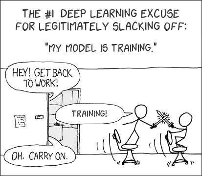
Image by Vishal Arora via medium
Lecture 5 Part 2 (Subgradient Descent): Link
Lecture 5 Part 3 (Kernel Trick): Link
Lecture 6 Part 1 (Decision Tree): Link
Lecture 6 Part 2 (Random Forrest): Link
Lecture 6 Part 3 (Nearest Neighbor): Link
Lecture 7 Part 1 (Convolution): Link
Lecture 7 Part 2 (Gradient Filters): Link
Lecture 7 Part 3 (Computer Vision): Link
Lecture 8 Part 1 (Computer Vision): Link
Lecture 8 Part 2 (Viola Jones): Link
Lecture 8 Part 3 (Convolutional Neural Net): Link
RBF Kernel SVM Demo: Link
Decision Tree: Link
Random Forrest Demo: Link
K Nearest Neighbor: Link
Map of Manhattan: Link
Voronoi Diagram: Link
KD Tree: Link
Image Filter: Link
Canny Edge Detection: Link
SIFT: PDF
HOG: PDF
Conv Net on MNIST: Link
Conv Net Vis: Link
LeNet: PDF, Link
Google Inception Net: PDF
CNN Architectures: Link
Image to Image: Link
Image segmentation: Link
Image colorization: Link, Link
Image Reconstruction: Link
Style Transfer: Link
Move Mirror: Link
Pose Estimation: Link
YOLO Attack: YouTube
Why does the kernel trick work? Link
Example (Quiz): Compute SVM classifier Link
Example (Quiz): Kernel SVM for XOR operator Link
Example (Quiz): Kernel matrix to feature vector Link
Example (Quiz): Entropy computation Link
Example (Quiz): Decision tree for implication operator Link
Example (Quiz): Three nearest neighbor Link
How to find the HOG features? Link
How to count the number of weights for training for a convolutional neural network (LeNet)? Link
Example (Quiz): How to find the 2D convolution between two matrices? Link
Example (Homework): How to find a discrete approximate Gausian filter? Link
Hard margin, original max-margin formulation: \(\displaystyle\max_{w} \dfrac{2}{\sqrt{w^\top w}}\) such that \(w^\top x_{i} + b \leq -1\) if \(y_{i} = 0\) and \(w^\top x_{i} + b \geq 1\) if \(y_{i} = 1\).
Hard margin, simplified formulation: \(\displaystyle\min_{w} \dfrac{1}{2} w^\top w\) such that \(\left(2 y_{i} - 1\right)\left(w^\top x_{i} + b\right) \geq 1\).
Soft margin, original max-margin formulation: \(\displaystyle\min_{w} \dfrac{1}{2} w^\top w + \dfrac{1}{\lambda} \dfrac{1}{n} \displaystyle\sum_{i=1}^{n} \xi_{i}\) such that \(\left(2 y_{i} - 1\right)\left(w^\top x_{i} + b\right) \geq 1 - \xi, \xi \geq 0\), where \(\xi_{i}\) is the slack variable for instance \(i\), \(\lambda\) is the regularization parameter.
Soft margin, simplified formulation: \(\displaystyle\min_{w} \dfrac{\lambda}{2} w^\top w + \dfrac{1}{n} \displaystyle\sum_{i=1}^{n} \displaystyle\max\left\{0, 1 - \left(2 y_{i} - 1\right) \left(w^\top x_{i} + b\right)\right\}\)
Subgradient descent formula: \(w = \left(1 - \lambda\right) w - \alpha \left(2 y_{i} - 1\right) 1_{\left\{\left(2 y_{i} - 1\right) \left(w^\top x_{i} + b\right) \geq 1\right\}} x_{i}\).
Kernal Gram matrix: \(K_{i i'} = \varphi\left(x_{i}\right)^\top \varphi\left(x_{i'}\right)\).
Quadratic Kernel: \(K_{i i'} = \left(x_{i^\top} x_{i'} + 1\right)^{2}\) has feature representation \(\varphi\left(x_{i}\right) = \left(x_{i1}^{2}, x_{i2}^{2}, \sqrt{2} x_{i1} x_{i2}, \sqrt{2} x_{i1}, \sqrt{2} x_{i2}, 1\right)\).
Gaussian RBF Kernel: \(K_{i i'} = \exp\left(- \dfrac{1}{2 \sigma^{2}} \left(x_{i} - x_{i'}\right)^\top \left(x_{i} - x_{i'}\right)\right)\) has infinite-dimensional feature representation, where \(\sigma^{2}\) is the variance parameter.
Conditional entropy: \(H\left(Y | X\right) = -\displaystyle\sum_{x=1}^{K_{X}} p_{x} \displaystyle\sum_{y=1}^{K} p_{y|x} \log_{2} \left(p_{y|x}\right)\), where \(K_{X}\) is the number of possible values of feature, \(p_{x}\) is the fraction of data points with feature \(x\), \(p_{y|x}\) is the fraction of data points with label \(y\) among the ones with feature \(x\).
Information gain, for feature \(j\): \(I\left(Y | X_{j}\right) = H\left(Y\right) - H\left(Y | X_{j}\right)\).
Feature selection: \(j^\star = \mathop{\mathrm{argmax}}_{j} I\left(Y | X_{j}\right)\).
Convolution (2D): \(A = X \star W\), \(A_{j j'} = \displaystyle\sum_{s=-k}^{k} \displaystyle\sum_{t=-k}^{k} W_{s,t} X_{j-s,j'-t}\), where \(W\) is the filter, and \(k\) is half of the width of the filter.
Sobel filter: \(W_{x} = \begin{bmatrix} -1 & 0 & 1 \\ -2 & 0 & 2 \\ -1 & 0 & 1 \end{bmatrix}\) and \(W_{y} = \begin{bmatrix} -1 & -2 & -1 \\ 0 & 0 & 0 \\ 1 & 2 & 1 \end{bmatrix}\).
Image gradient: \(\nabla_{x} X = W_{x} \star X\), \(\nabla_{y} X = W_{y} \star X\), with gradient magnitude \(G = \sqrt{\nabla_{x}^{2} + \nabla_{y}^{2}}\) and gradient direction \(\Theta = arctan\left(\dfrac{\nabla_{y}}{\nabla_{x}}\right)\).
Convolution layer: \(A = g\left(W \star X + b\right)\), where \(A\) is the activation map.
Pooling layer: (max-pooling) \(a = \displaystyle\max\left\{x_{1}, ..., x_{m}\right\}\), (average-pooling) \(a = \dfrac{1}{m} \displaystyle\sum_{j=1}^{m} x_{j}\).
# Summary
📗 Tuesday to Friday lectures: 1:00 to 2:15, Zoom Link
📗 Saturday review sessions: 5:30 to 8:30, Zoom Link
📗 Personal meeting room: always open, Zoom Link
📗 Quiz (use your wisc ID to log in (without "@wisc.edu")): Socrative Link
📗 Math Homework:
M4,
M5,
📗 Programming Homework:
P2,
📗 Examples and Quizzes:
Q5,
Q6,
Q7,
Q8,
# Lectures
📗 Slides (before lecture, usually updated on Sunday):
Blank Slides:
Part 1,
Part 2,
Part 3,
Part 4,
Blank Slides (with blank pages for quiz questions): Part 1, Part 2, Part 3, Part 4,
📗 Slides (after lecture, usually updated on Friday):
Blank Slides with Quiz Questions:
Part 1,
Part 2,
Part 3,
Part 4,
Annotated Slides: Part 1, Part 2, Part 3, Part 4,
📗 Review Session:
PDF. 📗 My handwriting is really bad, you should copy down your notes from the lecture videos instead of using these.
📗 Notes

Image by Vishal Arora via medium
# Other Materials
📗 Pre-recorded Videos from 2020
Lecture 5 Part 1 (Support Vector Machines): Link Lecture 5 Part 2 (Subgradient Descent): Link
Lecture 5 Part 3 (Kernel Trick): Link
Lecture 6 Part 1 (Decision Tree): Link
Lecture 6 Part 2 (Random Forrest): Link
Lecture 6 Part 3 (Nearest Neighbor): Link
Lecture 7 Part 1 (Convolution): Link
Lecture 7 Part 2 (Gradient Filters): Link
Lecture 7 Part 3 (Computer Vision): Link
Lecture 8 Part 1 (Computer Vision): Link
Lecture 8 Part 2 (Viola Jones): Link
Lecture 8 Part 3 (Convolutional Neural Net): Link
📗 Relevant websites
Support Vector Machine: Link RBF Kernel SVM Demo: Link
Decision Tree: Link
Random Forrest Demo: Link
K Nearest Neighbor: Link
Map of Manhattan: Link
Voronoi Diagram: Link
KD Tree: Link
Image Filter: Link
Canny Edge Detection: Link
SIFT: PDF
HOG: PDF
Conv Net on MNIST: Link
Conv Net Vis: Link
LeNet: PDF, Link
Google Inception Net: PDF
CNN Architectures: Link
Image to Image: Link
Image segmentation: Link
Image colorization: Link, Link
Image Reconstruction: Link
Style Transfer: Link
Move Mirror: Link
Pose Estimation: Link
YOLO Attack: YouTube
📗 YouTube videos from 2019 and 2020
How to find the margin expression for SVM? Link Why does the kernel trick work? Link
Example (Quiz): Compute SVM classifier Link
Example (Quiz): Kernel SVM for XOR operator Link
Example (Quiz): Kernel matrix to feature vector Link
Example (Quiz): Entropy computation Link
Example (Quiz): Decision tree for implication operator Link
Example (Quiz): Three nearest neighbor Link
How to find the HOG features? Link
How to count the number of weights for training for a convolutional neural network (LeNet)? Link
Example (Quiz): How to find the 2D convolution between two matrices? Link
Example (Homework): How to find a discrete approximate Gausian filter? Link
# Keywords and Notations
📗 Support Vector Machine
SVM classifier: \(\hat{y}_{i} = 1_{\left\{w^\top x_{i} + b \geq 0\right\}}\). Hard margin, original max-margin formulation: \(\displaystyle\max_{w} \dfrac{2}{\sqrt{w^\top w}}\) such that \(w^\top x_{i} + b \leq -1\) if \(y_{i} = 0\) and \(w^\top x_{i} + b \geq 1\) if \(y_{i} = 1\).
Hard margin, simplified formulation: \(\displaystyle\min_{w} \dfrac{1}{2} w^\top w\) such that \(\left(2 y_{i} - 1\right)\left(w^\top x_{i} + b\right) \geq 1\).
Soft margin, original max-margin formulation: \(\displaystyle\min_{w} \dfrac{1}{2} w^\top w + \dfrac{1}{\lambda} \dfrac{1}{n} \displaystyle\sum_{i=1}^{n} \xi_{i}\) such that \(\left(2 y_{i} - 1\right)\left(w^\top x_{i} + b\right) \geq 1 - \xi, \xi \geq 0\), where \(\xi_{i}\) is the slack variable for instance \(i\), \(\lambda\) is the regularization parameter.
Soft margin, simplified formulation: \(\displaystyle\min_{w} \dfrac{\lambda}{2} w^\top w + \dfrac{1}{n} \displaystyle\sum_{i=1}^{n} \displaystyle\max\left\{0, 1 - \left(2 y_{i} - 1\right) \left(w^\top x_{i} + b\right)\right\}\)
Subgradient descent formula: \(w = \left(1 - \lambda\right) w - \alpha \left(2 y_{i} - 1\right) 1_{\left\{\left(2 y_{i} - 1\right) \left(w^\top x_{i} + b\right) \geq 1\right\}} x_{i}\).
📗 Kernel Trick
Kernel SVM classifier: \(\hat{y}_{i} = 1_{\left\{w^\top \varphi\left(x_{i}\right) + b \geq 0\right\}}\), where \(\varphi\) is the feature map. Kernal Gram matrix: \(K_{i i'} = \varphi\left(x_{i}\right)^\top \varphi\left(x_{i'}\right)\).
Quadratic Kernel: \(K_{i i'} = \left(x_{i^\top} x_{i'} + 1\right)^{2}\) has feature representation \(\varphi\left(x_{i}\right) = \left(x_{i1}^{2}, x_{i2}^{2}, \sqrt{2} x_{i1} x_{i2}, \sqrt{2} x_{i1}, \sqrt{2} x_{i2}, 1\right)\).
Gaussian RBF Kernel: \(K_{i i'} = \exp\left(- \dfrac{1}{2 \sigma^{2}} \left(x_{i} - x_{i'}\right)^\top \left(x_{i} - x_{i'}\right)\right)\) has infinite-dimensional feature representation, where \(\sigma^{2}\) is the variance parameter.
📗 Information Theory:
Entropy: \(H\left(Y\right) = -\displaystyle\sum_{y=1}^{K} p_{y} \log_{2} \left(p_{y}\right)\), where \(K\) is the number of classes (number of possible labels), \(p_{y}\) is the fraction of data points with label \(y\). Conditional entropy: \(H\left(Y | X\right) = -\displaystyle\sum_{x=1}^{K_{X}} p_{x} \displaystyle\sum_{y=1}^{K} p_{y|x} \log_{2} \left(p_{y|x}\right)\), where \(K_{X}\) is the number of possible values of feature, \(p_{x}\) is the fraction of data points with feature \(x\), \(p_{y|x}\) is the fraction of data points with label \(y\) among the ones with feature \(x\).
Information gain, for feature \(j\): \(I\left(Y | X_{j}\right) = H\left(Y\right) - H\left(Y | X_{j}\right)\).
📗 Decision Tree:
Decision stump classifier: \(\hat{y}_{i} = 1_{\left\{x_{ij} \geq t_{j}\right\}}\), where \(t_{j}\) is the threshold for feature \(j\). Feature selection: \(j^\star = \mathop{\mathrm{argmax}}_{j} I\left(Y | X_{j}\right)\).
📗 Convolution
Convolution (1D): \(a = x \star w\), \(a_{j} = \displaystyle\sum_{t=-k}^{k} w_{t} x_{j-t}\), where \(w\) is the filter, and \(k\) is half of the width of the filter. Convolution (2D): \(A = X \star W\), \(A_{j j'} = \displaystyle\sum_{s=-k}^{k} \displaystyle\sum_{t=-k}^{k} W_{s,t} X_{j-s,j'-t}\), where \(W\) is the filter, and \(k\) is half of the width of the filter.
Sobel filter: \(W_{x} = \begin{bmatrix} -1 & 0 & 1 \\ -2 & 0 & 2 \\ -1 & 0 & 1 \end{bmatrix}\) and \(W_{y} = \begin{bmatrix} -1 & -2 & -1 \\ 0 & 0 & 0 \\ 1 & 2 & 1 \end{bmatrix}\).
Image gradient: \(\nabla_{x} X = W_{x} \star X\), \(\nabla_{y} X = W_{y} \star X\), with gradient magnitude \(G = \sqrt{\nabla_{x}^{2} + \nabla_{y}^{2}}\) and gradient direction \(\Theta = arctan\left(\dfrac{\nabla_{y}}{\nabla_{x}}\right)\).
📗 Convolutional Neural Network
Fully connected layer: \(a = g\left(w^\top x + b\right)\), where \(a\) is the activation unit, \(g\) is the activation function. Convolution layer: \(A = g\left(W \star X + b\right)\), where \(A\) is the activation map.
Pooling layer: (max-pooling) \(a = \displaystyle\max\left\{x_{1}, ..., x_{m}\right\}\), (average-pooling) \(a = \dfrac{1}{m} \displaystyle\sum_{j=1}^{m} x_{j}\).
Last Updated: April 19, 2026 at 1:55 AM