Prev: W2 Next: W4
Blank Slides (with blank pages for quiz questions): Part 1, Part 2, Part 3,
Annotated Slides: Part 1, Part 2, Part 3,

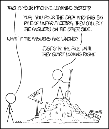
Image by xkcd via towards data science
Lecture 10 Part 2 (Natural Language): Link
Lecture 10 Part 3 (Sampling): Link
Lecture 11 Part 1 (Probability Distribution): Link
Lecture 11 Part 2 (Bayesian Network): Link
Lecture 11 Part 3 (Network Structure): Link
Lecture 11 Part 4 (Naive Bayes): Link
Lecture 12 Part 1 (Hidden Markov Model): Link
Lecture 12 Part 2 (HMM Evaluation): Link
Lecture 12 Part 3 (HMM Training): Link
Lecture 12 Part 4 (Recurrent Neural Network): Link
Lecture 12 Part 5 (Backprop Through Time): Link
Lecture 12 Part 6 (RNN Variants): Link
Markov Chain: Link
Google N-Gram: Link
Simple Bayes Net: Link, Link 2
ABNMS: Link, pathfinder: Link
RNN Visualization: Link
LTSM and GRU: Link
How to generate realizations of discrete random variables using CDF inversion? Link
Example: How to compute the joint probability given the conditional probability table? Link
Example (Quiz): How to compute conditional probability table given training data? Link
Example (Quiz): How to do inference (find joint and conditional probability) given conditional probability table? Link
Example (Quiz): How to find the conditional probabilities for a common cause configuration? Link
K-Nearest Neighbor classifier: \(\hat{y}_{i}\) = mode \(\left\{y_{\left(1\right)}, y_{\left(2\right)}, ..., y_{\left(k\right)}\right\}\), where mode is the majority label and \(y_{\left(t\right)}\) is the label of the \(t\)-th closest instance to instance \(i\) from the training set.
Maximum likelihood estimator (unigram): \(\hat{\mathbb{P}}\left\{z_{t}\right\} = \dfrac{c_{z_{t}}}{\displaystyle\sum_{z=1}^{m} c_{z}}\), where \(c_{z}\) is the number of time the token \(z\) appears in the training set and \(m\) is the vocabulary size (number of unique tokens).
Maximum likelihood estimator (unigram, with Laplace smoothing): \(\hat{\mathbb{P}}\left\{z_{t}\right\} = \dfrac{c_{z_{t}} + 1}{\left(\displaystyle\sum_{z=1}^{m} c_{z}\right) + m}\).
Bigram model: \(\mathbb{P}\left\{z_{1}, z_{2}, ..., z_{d}\right\} = \mathbb{P}\left\{z_{1}\right\} \displaystyle\prod_{t=2}^{d} \mathbb{P}\left\{z_{t} | z_{t-1}\right\}\).
Maximum likelihood estimator (bigram): \(\hat{\mathbb{P}}\left\{z_{t} | z_{t-1}\right\} = \dfrac{c_{z_{t-1}, z_{t}}}{c_{z_{t-1}}}\).
Maximum likelihood estimator (bigram, with Laplace smoothing): \(\hat{\mathbb{P}}\left\{z_{t} | z_{t-1}\right\} = \dfrac{c_{z_{t-1}, z_{t}} + 1}{c_{z_{t-1}} + m}\).
Joint probability: \(\mathbb{P}\left\{X = x\right\} = \displaystyle\sum_{y \in Y} \mathbb{P}\left\{X = x, Y = y\right\}\).
Bayes rule: \(\mathbb{P}\left\{Y = y | X = x\right\} = \dfrac{\mathbb{P}\left\{X = x | Y = y\right\} \mathbb{P}\left\{Y = y\right\}}{\displaystyle\sum_{y' \in Y} \mathbb{P}\left\{X = x | Y = y'\right\} \mathbb{P}\left\{Y = y'\right\}}\).
Law of total probability: \(\mathbb{P}\left\{X = x\right\} = \displaystyle\sum_{y' \in Y} \mathbb{P}\left\{X = x | Y = y'\right\} \mathbb{P}\left\{Y = y'\right\}\).
Independence: \(X, Y\) are independent if \(\mathbb{P}\left\{X = x, Y = y\right\} = \mathbb{P}\left\{X = x\right\} \mathbb{P}\left\{Y = y\right\}\) for every \(x, y\).
Conditional independence: \(X, Y\) are conditionally independent conditioned on \(Z\) if \(\mathbb{P}\left\{X = x, Y = y | Z = z\right\} = \mathbb{P}\left\{X = x | Z = z\right\} \mathbb{P}\left\{Y = y | Z = z\right\}\) for every \(x, y, z\).
Conditional Probability Table estimation (with Laplace smoothing): \(\hat{\mathbb{P}}\left\{x_{j} | p\left(X_{j}\right)\right\} = \dfrac{c_{x_{j}, p\left(X_{j}\right)} + 1}{c_{p\left(X_{j}\right)} + \left| X_{j} \right|}\), where \(\left| X_{j} \right|\) is the number of possible values of \(X_{j}\).
Bayesian network inference: \(\mathbb{P}\left\{x_{1}, x_{2}, ..., x_{m}\right\} = \displaystyle\prod_{j=1}^{m} \mathbb{P}\left\{x_{j} | p\left(X_{j}\right)\right\}\).
Naive Bayes estimation: .
Naive Bayes classifier: \(\hat{y}_{i} = \mathop{\mathrm{argmax}}_{y} \mathbb{P}\left\{Y = y | X = X_{i}\right\}\).
# Summary
📗 Tuesday to Friday lectures: 1:00 to 2:15, Zoom Link
📗 Saturday review sessions: 5:30 to 8:30, Zoom Link
📗 Personal meeting room: always open, Zoom Link
📗 Quiz (use your wisc ID to log in (without "@wisc.edu")): Socrative Link
📗 Math Homework:
M6,
M7,
📗 Programming Homework:
P3,
P6,
📗 Examples and Quizzes:
Q9,
Q10,
Q11,
Q12,
Q13,
Q14,
# Lectures
📗 Slides (before lecture, usually updated on Sunday):
Blank Slides:
Part 1,
Part 2,
Part 3,
Blank Slides (with blank pages for quiz questions): Part 1, Part 2, Part 3,
📗 Slides (after lecture, usually updated on Friday):
Blank Slides with Quiz Questions:
Part 1,
Part 2,
Part 3,
Annotated Slides: Part 1, Part 2, Part 3,
📗 Review Session:
PDF. 📗 My handwriting is really bad, you should copy down your notes from the lecture videos instead of using these.
📗 Notes

Image by xkcd via towards data science
# Other Materials
📗 Pre-recorded Videos from 2020
Lecture 10 Part 1 (Generative Models): Link Lecture 10 Part 2 (Natural Language): Link
Lecture 10 Part 3 (Sampling): Link
Lecture 11 Part 1 (Probability Distribution): Link
Lecture 11 Part 2 (Bayesian Network): Link
Lecture 11 Part 3 (Network Structure): Link
Lecture 11 Part 4 (Naive Bayes): Link
Lecture 12 Part 1 (Hidden Markov Model): Link
Lecture 12 Part 2 (HMM Evaluation): Link
Lecture 12 Part 3 (HMM Training): Link
Lecture 12 Part 4 (Recurrent Neural Network): Link
Lecture 12 Part 5 (Backprop Through Time): Link
Lecture 12 Part 6 (RNN Variants): Link
📗 Relevant websites
Zipf's Law: Link Markov Chain: Link
Google N-Gram: Link
Simple Bayes Net: Link, Link 2
ABNMS: Link, pathfinder: Link
RNN Visualization: Link
LTSM and GRU: Link
📗 YouTube videos from 2019 and 2020
How to find maximum likelihood estimates for Bernoulli distribution? Link How to generate realizations of discrete random variables using CDF inversion? Link
Example: How to compute the joint probability given the conditional probability table? Link
Example (Quiz): How to compute conditional probability table given training data? Link
Example (Quiz): How to do inference (find joint and conditional probability) given conditional probability table? Link
Example (Quiz): How to find the conditional probabilities for a common cause configuration? Link
# Keywords and Notations
📗 K-Nearest Neighbor:
Distance: (Euclidean) \(\rho\left(x, x'\right) = \left\|x - x'\right\|_{2} = \sqrt{\displaystyle\sum_{j=1}^{m} \left(x_{j} - x'_{j}\right)^{2}}\), (Manhattan) \(\rho\left(x, x'\right) = \left\|x - x'\right\|_{1} = \displaystyle\sum_{j=1}^{m} \left| x_{j} - x'_{j} \right|\), where \(x, x'\) are two instances. K-Nearest Neighbor classifier: \(\hat{y}_{i}\) = mode \(\left\{y_{\left(1\right)}, y_{\left(2\right)}, ..., y_{\left(k\right)}\right\}\), where mode is the majority label and \(y_{\left(t\right)}\) is the label of the \(t\)-th closest instance to instance \(i\) from the training set.
📗 Natural Language Processing:
Unigram model: \(\mathbb{P}\left\{z_{1}, z_{2}, ..., z_{d}\right\} = \displaystyle\prod_{t=1}^{d} \mathbb{P}\left\{z_{t}\right\}\) where \(z_{t}\) is the \(t\)-th token in a training item, and \(d\) is the total number of tokens in the item. Maximum likelihood estimator (unigram): \(\hat{\mathbb{P}}\left\{z_{t}\right\} = \dfrac{c_{z_{t}}}{\displaystyle\sum_{z=1}^{m} c_{z}}\), where \(c_{z}\) is the number of time the token \(z\) appears in the training set and \(m\) is the vocabulary size (number of unique tokens).
Maximum likelihood estimator (unigram, with Laplace smoothing): \(\hat{\mathbb{P}}\left\{z_{t}\right\} = \dfrac{c_{z_{t}} + 1}{\left(\displaystyle\sum_{z=1}^{m} c_{z}\right) + m}\).
Bigram model: \(\mathbb{P}\left\{z_{1}, z_{2}, ..., z_{d}\right\} = \mathbb{P}\left\{z_{1}\right\} \displaystyle\prod_{t=2}^{d} \mathbb{P}\left\{z_{t} | z_{t-1}\right\}\).
Maximum likelihood estimator (bigram): \(\hat{\mathbb{P}}\left\{z_{t} | z_{t-1}\right\} = \dfrac{c_{z_{t-1}, z_{t}}}{c_{z_{t-1}}}\).
Maximum likelihood estimator (bigram, with Laplace smoothing): \(\hat{\mathbb{P}}\left\{z_{t} | z_{t-1}\right\} = \dfrac{c_{z_{t-1}, z_{t}} + 1}{c_{z_{t-1}} + m}\).
📗 Probability Review:
Conditional probability: \(\mathbb{P}\left\{Y = y | X = x\right\} = \dfrac{\mathbb{P}\left\{Y = y, X = x\right\}}{\mathbb{P}\left\{X = x\right\}}\). Joint probability: \(\mathbb{P}\left\{X = x\right\} = \displaystyle\sum_{y \in Y} \mathbb{P}\left\{X = x, Y = y\right\}\).
Bayes rule: \(\mathbb{P}\left\{Y = y | X = x\right\} = \dfrac{\mathbb{P}\left\{X = x | Y = y\right\} \mathbb{P}\left\{Y = y\right\}}{\displaystyle\sum_{y' \in Y} \mathbb{P}\left\{X = x | Y = y'\right\} \mathbb{P}\left\{Y = y'\right\}}\).
Law of total probability: \(\mathbb{P}\left\{X = x\right\} = \displaystyle\sum_{y' \in Y} \mathbb{P}\left\{X = x | Y = y'\right\} \mathbb{P}\left\{Y = y'\right\}\).
Independence: \(X, Y\) are independent if \(\mathbb{P}\left\{X = x, Y = y\right\} = \mathbb{P}\left\{X = x\right\} \mathbb{P}\left\{Y = y\right\}\) for every \(x, y\).
Conditional independence: \(X, Y\) are conditionally independent conditioned on \(Z\) if \(\mathbb{P}\left\{X = x, Y = y | Z = z\right\} = \mathbb{P}\left\{X = x | Z = z\right\} \mathbb{P}\left\{Y = y | Z = z\right\}\) for every \(x, y, z\).
📗 Bayesian Network
Conditional Probability Table estimation: \(\hat{\mathbb{P}}\left\{x_{j} | p\left(X_{j}\right)\right\} = \dfrac{c_{x_{j}, p\left(X_{j}\right)}}{c_{p\left(X_{j}\right)}}\), where \(p\left(X_{j}\right)\) is the list of parents of \(X_{j}\) in the network. Conditional Probability Table estimation (with Laplace smoothing): \(\hat{\mathbb{P}}\left\{x_{j} | p\left(X_{j}\right)\right\} = \dfrac{c_{x_{j}, p\left(X_{j}\right)} + 1}{c_{p\left(X_{j}\right)} + \left| X_{j} \right|}\), where \(\left| X_{j} \right|\) is the number of possible values of \(X_{j}\).
Bayesian network inference: \(\mathbb{P}\left\{x_{1}, x_{2}, ..., x_{m}\right\} = \displaystyle\prod_{j=1}^{m} \mathbb{P}\left\{x_{j} | p\left(X_{j}\right)\right\}\).
Naive Bayes estimation: .
Naive Bayes classifier: \(\hat{y}_{i} = \mathop{\mathrm{argmax}}_{y} \mathbb{P}\left\{Y = y | X = X_{i}\right\}\).
Last Updated: April 19, 2026 at 1:55 AM