Prev: W3 Next: W5
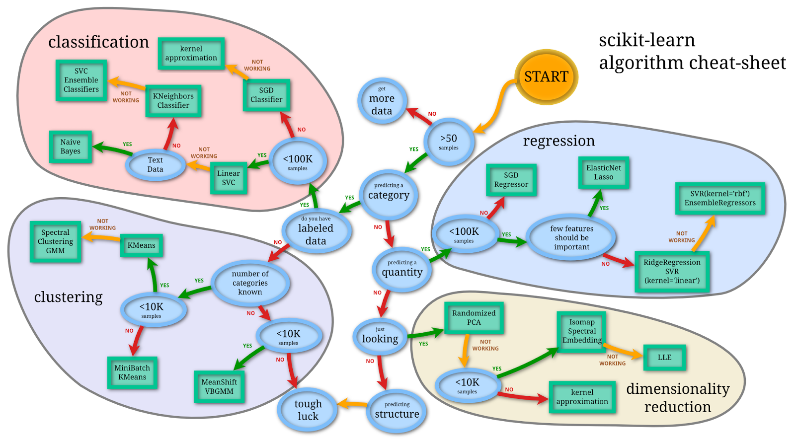
Image by scikit learn
W2 : M4 and M5
W3 : M6
Practice: X1 and X2 and X3 and X4
M2A Permutations: Link
M1B Permutations: Link
M2B Permutations: Link
M1A: Mean = 66.86%, Stdev = 20.95
M2A: Mean = 76.88%, Stdev = 16.22
M1B: Mean = 71.51%, Stdev = 23.13
M2B: Mean = 60.95%, Stdev = 27.79
(2) The slides subtitled "Motivation" and "Discussion" contain concepts you should be familiar with, but the specific mathematics will not be tested on the exam.
(3) The slides subtitled "Description" and "Algorithm" are mostly useful for programming homework, not exams.
(4) The slides subtitled "Admin" are not relevant to the course materials.
(2) Around a third of the questions will be similar to the homework or quiz or past exam questions (similar method to solve the problems).
(3) Around a third of the questions will be new, mostly from topics not covered in the homework, and reading the slides will be helpful.
Lecture 14 (Optimization): Guest Lecture (see Canvas Zoom recording)
EX1: Link
CX1: Link
CX2: Link
2023 Online Exams:
M1A: Link
M2A: Link
M1B: Link
M2B: Link
2022 Online Exams:
M1A-C: Link
M2A-C: Link
MB-C: Link
MA-E: Link
MB-E: Link
2021 Online Exams:
M1A-C: Link
M1B-C: Link
M2A-C: Link
M2B-C: Link
2020 Online Exams:
M1A-C: Link
M1B-C: Link
M2A-C: Link
M2B-C: Link
M1A-E: Link
M1B-E: Link
M2A-E: Link
M2B-E: Link
2019 In-person Exams:
Midterm Version A: Link
Version A Answers: ABEDE ECDDC CCBCC CEDBB CEECD DDDBC DBBAA AAADC
Midterm Version B: Link
Version B Answers: CCABD DAECE BCADC CCEBA DDCCD DDCCA AADBC ABDAB
Sample midterm: Link
Why cannot use linear regression for binary classification? Link
How to use Perceptron update formula? Link
How to find the size of the hypothesis space for linear classifiers? Link (Part 1)
Computation of Hessian of quadratic form Link
Computation of eigenvalues Link
Gradient descent for linear regression Link
What is the gradient descent step for cross-entropy loss with linear activation? Link (Part 1)
What is the sign of the next gradient descent step? Link (Part 2)
Which loss functions are equivalent to squared loss? Link (Part 3)
How to compute the gradient of the cross-entropy loss with linear activation? Link (Part 4)
How to find the location that minimizes the distance to multiple points? Link (Part 3)
Gradient descent for logistic activation with squared error Link
How to compute logistic gradient descent? Link
How derive 2-layer neural network gradient descent step? Link
How derive multi-layer neural network gradient descent induction step? Link
How to find the missing weights in neural network given data set? Link
How many weights are used in one step of backpropogation? Link (Part 2)
How to compute cross validation accuracy? Link
Compute SVM classifier Link
How to find the distance from a plane to a point? Link
How to find the formula for SVM given two training points? Link
What is the largest number of points that can be removed to maintain the same SVM? Link (Part 4)
What is minimum number of points that can be removed to improve the SVM margin? Link (Part 5)
How many training items are needed for a one-vs-one SVM? Link (Part 2)
Which items are used in a multi-lcass one-vs-one SVM? Link (Part 7)
How to compute the subgradient? Link (Part 2)
What happens if the lambda in soft-margin SVM is 0? Link (Part 3)
How to compute the hinge loss gradient? Link (Part 1)
How to find feature representation for sum of two kernel (Gram) matrices? Link
What is the kernel SVM for XOR operator? Link
How to convert the kernel matrix to feature vector? Link
How to find the kernel (Gram) matrix given the feature representation? Link (Part 1)
How to find the feature vector based on the kernel (Gram) matrix? Link (Part 4)
How to find the kernal (Gram) matrix based on the feature vectors? Link (Part 10)
How to find the information gain given two distributions (this is the Avatar question)? Link
What distribution maximizes the entropy? Link (Part 1)
How to create a dataset with information gain of 0? Link (Part 2)
How to compute the conditional entropy based on a binary variable dataset? Link (Part 3)
How to find conditional entropy given a dataset? Link (Part 9)
When is the information gain based on a dataset equal to zero? Link (Part 10)
How to compute entropy of a binary variable? Link (Part 1)
How to compute information gain, the Avatar question? Link (Part 2)
How to compute conditional entropy based on a training set? Link (Part 3)
How many conditional entropy calculations are needed for a decision tree with real-valued features? Link (Part 1)
What is the maximum and minimum training set accuracy for a decision tree? Link (Part 2)
How to find the minimum number of conditional entropies that need to be computed for a binary decision tree? Link (Part 9)
What is the maximum number of conditional entropies that need to be computed in a decision tree at a certain depth? Link (Part 4)
How to find a KNN decision boundary? Link
What is the accuracy for KNN when K = n or K = 1? Link (Part 1)
Which K maximizes the accuracy of KNN? Link (Part 3)
How to work with KNN with distance defined on the alphabet? Link (Part 4)
How to find the 1NN accuracy on training set? Link (Part 8)
How to draw the decision boundary of 1NN in 2D? Link (Part 1)
How to find the smallest k such that all items are classified as the same label with kNN? Link (Part 2)
Which value of k maximizes the accuracy of kNN? Link (Part 3)
What is the leave-one-out accuracy for KNN with K = n? Link (Part 2)
How to compute cross validation accuracy for KNN? Link (Part 5)
What is the leave-one-out accuracy for n-1-NN? Link (Part 5)
How to find the 3 fold cross validation accuracy of a 1NN classifier? Link (Part 12)
How to compute the convolution between a matrix an a gradient (Sobel) filter? Link (Part 2)
How to find the 2D convolution between two matrices? Link
How to find a discrete approximate Gausian filter? Link
How to find the HOG features? Link
How to compute the gradient magnitude of pixel? Link (Part 3)
How to compute the convolution of a 2D image with a Sobel filter? Link (Part 2)
How to compute the convolution of a 2D image with a 1D gradient filter? Link (Part 8)
How to compute the convolution of a 2D image with a sparse 2D filter? Link (Part 13)
How to find the gradient magnitude using Sobel filter? Link (Part 3)
How to find the gradient direction bin? Link (Part 4)
How to find the number of weights in a CNN? Link
How to compute the activation map after a pooling layer? Link (Part 1)
How to find the number of weights in a CNN? Link (Part 2)
How to compute the activation map after a max-pooling layer? Link (Part 11)
How many weights are there in a CNN? Link (Part 11)
How to find the number of weights and biases in a CNN? Link (Part 1)
How to find the activation map after a pooling layer? Link (Part 2)
How to compute the marginal probabilities given the ratio between the conditionals? Link (Part 1)
How to compute the conditional probabilities given the same variable? Link (Part 1)
What is the probability of switch between elements in a cycle? Link (Part 2)
Which marginal probabilities are valid given the joint probabilities? Link (Part 3)
How to use the Bayes rule to find which biased coin leads to a sequence of coin flips? Link
Please do NOT forget to submit your homework on Canvas! Link
How to use Bayes rule to find the probability of truth telling? Link (Part 6)
How to estimate fraction given randomized survey data? Link (Part 12)
How to write down the joint probability table given the variables are independent? Link (Part 13)
Given the ratio between two conditional probabilities, how to compute the marginal probabilities? Link (Part 1)
What is the Boy or Girl paradox? Link (Part 3)
How to compute the maximum likelihood estimate of a conditional probability given a count table? Link (Part 1)
How to compare the probabilities in the Boy or Girl Paradox? Link (Part 3)
How to find maximum likelihood estimates for Bernoulli distribution? Link
How to generate realizations of discrete random variables using CDF inversion? Link
How to find the sentence generated given the random number from CDF inversion? Link (Part 3)
How to find the probability of observing a sentence given the first and last word using the transition matrix? Link (Part 14)
How many conditional probabilities need to be stored for a n-gram model? Link (Part 2)
How to compute conditional probability table given training data? Link
How to do inference (find joint and conditional probability) given conditional probability table? Link
How to find the conditional probabilities for a common cause configuration? Link
What is the size of the conditional probability table? Link
How to compute a condition probability given a Bayesian network with three variables? Link
What is the size of a conditional probability table of two discrete variables? Link (Part 2)
How many joint probabilities are needed to compute a marginal probability? Link (Part 3)
How to compute the MLE conditional probability with Laplace smoothing given a data set? Link (Part 2)
What is the number of conditional probabilities stored in a CPT given a Bayesian network? Link (Part 3)
How to compute the number of probabilities in a CPT for variables with more than two possible values? Link (Part 14)
How to find the MLE of the conditional probability given the sum of two variables? Link (Part 5)
How many joint probabilities are used in the computation of a marginal probability? Link (Part 4)
How to find the size of an arbitrary Bayesian network with binary variables? Link (Part 3)
How to find the size of the conditional probability table for a Naive Bayes model? Link
How to compute the probability of observing a sequence under an HMM? Link
What is the number of conditional probabilities stored in a CPT given a Naive Bayes model? Link (Part 4)
How to find th obervation probabilities given an HMM? Link (Part 2)
What is the size of the CPT for a Naive Bayes network? Link (Part 1)
How to detect virus in email messages using Naive Bayes? Link (Part 2)
What is the relationship between Naive Bayes and Logistic Regression? Link
Test item: \(\left(x', y'\right)\), where \(j \in \left\{1, 2, ..., m\right\}\) is the feature index.
Perceptron algorithm update step: \(w = w - \alpha \left(a_{i} - y_{i}\right) x_{i}\), \(b = b - \alpha \left(a_{i} - y_{i}\right)\), \(a_{i} = 1_{\left\{w^\top x_{i} + b \geq 0\right\}}\), where \(a_{i}\) is the activation value of instance \(i\).
Squared loss minimization of perceptrons: \(\left(\hat{w}, \hat{b}\right) = \mathop{\mathrm{argmin}}_{w, b} \dfrac{1}{2} \displaystyle\sum_{i=1}^{n} \left(a_{i} - y_{i}\right)^{2}\), \(a_{i} = g\left(w^\top x_{i} + b\right)\), where \(\hat{w}\) is the optimal weights, \(\hat{b}\) is the optimal bias, \(g\) is the activation function.
Loss minimization problem: \(\left(\hat{w}, \hat{b}\right) = \mathop{\mathrm{argmin}}_{w, b} -\displaystyle\sum_{i=1}^{n} \left(y_{i} \log\left(a_{i}\right) + \left(1 - y_{i}\right) \log\left(1 - a_{i}\right)\right)\), \(a_{i} = \dfrac{1}{1 + \exp\left(- \left(w^\top x_{i} + b\right)\right)}\).
Batch gradient descrent step: \(w = w - \alpha \displaystyle\sum_{i=1}^{n} \left(a_{i} - y_{i}\right) x_{i}\), \(b = b - \alpha \displaystyle\sum_{i=1}^{n} \left(a_{i} - y_{i}\right)\), \(a_{i} = \dfrac{1}{1 + \exp\left(- \left(w^\top x_{i} + b\right)\right)}\), where \(\alpha\) is the learning rate.
\(a^{\left(1\right)}_{ij} = \dfrac{1}{1 + \exp\left(- \left(\left(\displaystyle\sum_{j'=1}^{m} x_{ij'} w^{\left(1\right)}_{j'j}\right) + b^{\left(1\right)}_{j}\right)\right)}\), where \(m\) is the number of features (or input units), \(w^{\left(1\right)}_{j' j}\) is the layer \(1\) weight from input unit \(j'\) to hidden layer unit \(j\), \(b^{\left(1\right)}_{j}\) is the bias for hidden layer unit \(j\), \(a_{ij}^{\left(1\right)}\) is the layer \(1\) activation of instance \(i\) hidden unit \(j\).
\(a^{\left(2\right)}_{i} = \dfrac{1}{1 + \exp\left(- \left(\left(\displaystyle\sum_{j=1}^{h} a^{\left(1\right)}_{ij} w^{\left(2\right)}_{j}\right) + b^{\left(2\right)}\right)\right)}\), where \(h\) is the number of hidden units, \(w^{\left(2\right)}_{j}\) is the layer \(2\) weight from hidden layer unit \(j\), \(b^{\left(2\right)}\) is the bias for the output unit, \(a^{\left(2\right)}_{i}\) is the layer \(2\) activation of instance \(i\).
Stochastic gradient descent step for two layer network with squared loss and logistic activation:
\(w^{\left(1\right)}_{j' j} = w^{\left(1\right)}_{j' j} - \alpha \left(a^{\left(2\right)}_{i} - y_{i}\right) a^{\left(2\right)}_{i} \left(1 - a^{\left(2\right)}_{i}\right) w_{j}^{\left(2\right)} a_{ij}^{\left(1\right)} \left(1 - a_{ij}^{\left(1\right)}\right) x_{ij'}\).
\(b^{\left(1\right)}_{j} \leftarrow b^{\left(1\right)}_{j} - \alpha \left(a^{\left(2\right)}_{i} - y_{i}\right) a^{\left(2\right)}_{i} \left(1 - a^{\left(2\right)}_{i}\right) w_{j}^{\left(2\right)} a_{ij}^{\left(1\right)} \left(1 - a_{ij}^{\left(1\right)}\right)\).
\(w^{\left(2\right)}_{j} \leftarrow w^{\left(2\right)}_{j} - \alpha \left(a^{\left(2\right)}_{i} - y_{i}\right) a^{\left(2\right)}_{i} \left(1 - a^{\left(2\right)}_{i}\right) a_{ij}^{\left(1\right)}\).
\(b^{\left(2\right)} \leftarrow b^{\left(2\right)} - \alpha \left(a^{\left(2\right)}_{i} - y_{i}\right) a^{\left(2\right)}_{i} \left(1 - a^{\left(2\right)}_{i}\right)\).
L2 regularization (sqaured loss): \(\displaystyle\sum_{i=1}^{n} \left(a_{i} - y_{i}\right)^{2} + \lambda \left(\displaystyle\sum_{j=1}^{m} \left(w_{j}\right)^{2} + b^{2}\right)\).
Hard margin, original max-margin formulation: \(\displaystyle\max_{w} \dfrac{2}{\sqrt{w^\top w}}\) such that \(w^\top x_{i} + b \leq -1\) if \(y_{i} = 0\) and \(w^\top x_{i} + b \geq 1\) if \(y_{i} = 1\).
Hard margin, simplified formulation: \(\displaystyle\min_{w} \dfrac{1}{2} w^\top w\) such that \(\left(2 y_{i} - 1\right)\left(w^\top x_{i} + b\right) \geq 1\).
Soft margin, original max-margin formulation: \(\displaystyle\min_{w} \dfrac{1}{2} w^\top w + \dfrac{1}{\lambda} \dfrac{1}{n} \displaystyle\sum_{i=1}^{n} \xi_{i}\) such that \(\left(2 y_{i} - 1\right)\left(w^\top x_{i} + b\right) \geq 1 - \xi, \xi \geq 0\), where \(\xi_{i}\) is the slack variable for instance \(i\), \(\lambda\) is the regularization parameter.
Soft margin, simplified formulation: \(\displaystyle\min_{w} \dfrac{\lambda}{2} w^\top w + \dfrac{1}{n} \displaystyle\sum_{i=1}^{n} \displaystyle\max\left\{0, 1 - \left(2 y_{i} - 1\right) \left(w^\top x_{i} + b\right)\right\}\)
Subgradient descent formula: \(w = \left(1 - \lambda\right) w - \alpha \left(2 y_{i} - 1\right) 1_{\left\{\left(2 y_{i} - 1\right) \left(w^\top x_{i} + b\right) \geq 1\right\}} x_{i}\).
Kernal Gram matrix: \(K_{i i'} = \varphi\left(x_{i}\right)^\top \varphi\left(x_{i'}\right)\).
Quadratic Kernel: \(K_{i i'} = \left(x_{i^\top} x_{i'} + 1\right)^{2}\) has feature representation \(\varphi\left(x_{i}\right) = \left(x_{i1}^{2}, x_{i2}^{2}, \sqrt{2} x_{i1} x_{i2}, \sqrt{2} x_{i1}, \sqrt{2} x_{i2}, 1\right)\).
Gaussian RBF Kernel: \(K_{i i'} = \exp\left(- \dfrac{1}{2 \sigma^{2}} \left(x_{i} - x_{i'}\right)^\top \left(x_{i} - x_{i'}\right)\right)\) has infinite-dimensional feature representation, where \(\sigma^{2}\) is the variance parameter.
Conditional entropy: \(H\left(Y | X\right) = -\displaystyle\sum_{x=1}^{K_{X}} p_{x} \displaystyle\sum_{y=1}^{K} p_{y|x} \log_{2} \left(p_{y|x}\right)\), where \(K_{X}\) is the number of possible values of feature, \(p_{x}\) is the fraction of data points with feature \(x\), \(p_{y|x}\) is the fraction of data points with label \(y\) among the ones with feature \(x\).
Information gain, for feature \(j\): \(I\left(Y | X_{j}\right) = H\left(Y\right) - H\left(Y | X_{j}\right)\).
Feature selection: \(j^\star = \mathop{\mathrm{argmax}}_{j} I\left(Y | X_{j}\right)\).
K-Nearest Neighbor classifier: \(\hat{y}_{i}\) = mode \(\left\{y_{\left(1\right)}, y_{\left(2\right)}, ..., y_{\left(k\right)}\right\}\), where mode is the majority label and \(y_{\left(t\right)}\) is the label of the \(t\)-th closest instance to instance \(i\) from the training set.
Maximum likelihood estimator (unigram): \(\hat{\mathbb{P}}\left\{z_{t}\right\} = \dfrac{c_{z_{t}}}{\displaystyle\sum_{z=1}^{m} c_{z}}\), where \(c_{z}\) is the number of time the token \(z\) appears in the training set and \(m\) is the vocabulary size (number of unique tokens).
Maximum likelihood estimator (unigram, with Laplace smoothing): \(\hat{\mathbb{P}}\left\{z_{t}\right\} = \dfrac{c_{z_{t}} + 1}{\left(\displaystyle\sum_{z=1}^{m} c_{z}\right) + m}\).
Bigram model: \(\mathbb{P}\left\{z_{1}, z_{2}, ..., z_{d}\right\} = \mathbb{P}\left\{z_{1}\right\} \displaystyle\prod_{t=2}^{d} \mathbb{P}\left\{z_{t} | z_{t-1}\right\}\).
Maximum likelihood estimator (bigram): \(\hat{\mathbb{P}}\left\{z_{t} | z_{t-1}\right\} = \dfrac{c_{z_{t-1}, z_{t}}}{c_{z_{t-1}}}\).
Maximum likelihood estimator (bigram, with Laplace smoothing): \(\hat{\mathbb{P}}\left\{z_{t} | z_{t-1}\right\} = \dfrac{c_{z_{t-1}, z_{t}} + 1}{c_{z_{t-1}} + m}\).
Joint probability: \(\mathbb{P}\left\{X = x\right\} = \displaystyle\sum_{y \in Y} \mathbb{P}\left\{X = x, Y = y\right\}\).
Bayes rule: \(\mathbb{P}\left\{Y = y | X = x\right\} = \dfrac{\mathbb{P}\left\{X = x | Y = y\right\} \mathbb{P}\left\{Y = y\right\}}{\displaystyle\sum_{y' \in Y} \mathbb{P}\left\{X = x | Y = y'\right\} \mathbb{P}\left\{Y = y'\right\}}\).
Law of total probability: \(\mathbb{P}\left\{X = x\right\} = \displaystyle\sum_{y' \in Y} \mathbb{P}\left\{X = x | Y = y'\right\} \mathbb{P}\left\{Y = y'\right\}\).
Independence: \(X, Y\) are independent if \(\mathbb{P}\left\{X = x, Y = y\right\} = \mathbb{P}\left\{X = x\right\} \mathbb{P}\left\{Y = y\right\}\) for every \(x, y\).
Conditional independence: \(X, Y\) are conditionally independent conditioned on \(Z\) if \(\mathbb{P}\left\{X = x, Y = y | Z = z\right\} = \mathbb{P}\left\{X = x | Z = z\right\} \mathbb{P}\left\{Y = y | Z = z\right\}\) for every \(x, y, z\).
Conditional Probability Table estimation (with Laplace smoothing): \(\hat{\mathbb{P}}\left\{x_{j} | p\left(X_{j}\right)\right\} = \dfrac{c_{x_{j}, p\left(X_{j}\right)} + 1}{c_{p\left(X_{j}\right)} + \left| X_{j} \right|}\), where \(\left| X_{j} \right|\) is the number of possible values of \(X_{j}\).
Bayesian network inference: \(\mathbb{P}\left\{x_{1}, x_{2}, ..., x_{m}\right\} = \displaystyle\prod_{j=1}^{m} \mathbb{P}\left\{x_{j} | p\left(X_{j}\right)\right\}\).
Naive Bayes estimation: .
Naive Bayes classifier: \(\hat{y}_{i} = \mathop{\mathrm{argmax}}_{y} \mathbb{P}\left\{Y = y | X = X_{i}\right\}\).
Convolution (2D): \(A = X \star W\), \(A_{j j'} = \displaystyle\sum_{s=-k}^{k} \displaystyle\sum_{t=-k}^{k} W_{s,t} X_{j-s,j'-t}\), where \(W\) is the filter, and \(k\) is half of the width of the filter.
Sobel filter: \(W_{x} = \begin{bmatrix} -1 & 0 & 1 \\ -2 & 0 & 2 \\ -1 & 0 & 1 \end{bmatrix}\) and \(W_{y} = \begin{bmatrix} -1 & -2 & -1 \\ 0 & 0 & 0 \\ 1 & 2 & 1 \end{bmatrix}\).
Image gradient: \(\nabla_{x} X = W_{x} \star X\), \(\nabla_{y} X = W_{y} \star X\), with gradient magnitude \(G = \sqrt{\nabla_{x}^{2} + \nabla_{y}^{2}}\) and gradient direction \(\Theta = arctan\left(\dfrac{\nabla_{y}}{\nabla_{x}}\right)\).
Convolution layer: \(A = g\left(W \star X + b\right)\), where \(A\) is the activation map.
Pooling layer: (max-pooling) \(a = \displaystyle\max\left\{x_{1}, ..., x_{m}\right\}\), (average-pooling) \(a = \dfrac{1}{m} \displaystyle\sum_{j=1}^{m} x_{j}\).
# Summary
📗 Tuesday to Friday lectures: 1:00 to 2:15, Zoom Link
📗 Monday to Saturday office hours: Zoom Link
📗 Personal meeting room: always open, Zoom Link
📗 Math Homework:
M2,
M3,
M4,
M5,
M6,
📗 Programming Homework:
P1,
P2,
P3,
📗 Examples and Quizzes:
Q1,
Q2,
Q3,
Q4,
Q5,
Q6,
Q7,
Q8,
Q9,
Q10,
Q11,
Q12,
Q13,
Q14,
📗 Discussions:
D1,
D2,
D3,
D4,
D5,
D6,
# Lectures
📗 Slides (will be posted before lecture, usually updated on Monday):
Blank Slides:
Part 1: PDF,
Part 2: PDF,
📗 The annotated lecture slides will not be posted this year: please copy down the notes during the lecture or from the Zoom recording.
📗 Notes
Image by scikit learn
# Summary
📗 Coverage: supervised learning W1 to W4.
📗 Number of questions: 30
📗 Length: 2 x 1 hour 30 minutes
📗 Regular: July 13 AND July 14, 1:00 to 2:30 PM
📗 Make-up: July 13 AND July 14, 9:00 to 10:30 PM
📗 Link to relevant pages:
W1 : M2 and M3 W2 : M4 and M5
W3 : M6
Practice: X1 and X2 and X3 and X4
# Exams
M1A Permutations: LinkM2A Permutations: Link
M1B Permutations: Link
M2B Permutations: Link
M1A: Mean = 66.86%, Stdev = 20.95
| Q | 1 | 2 | 3 | 4 | 5 | 6 | 7 | 8 | 9 | 10 | 11 | 12 | 13 | 14 | 15 |
| MAX | 2 | 4 | 3 | 4 | 4 | 2 | 3 | 4 | 4 | 4 | 4 | 2 | 4 | 4 | 1 |
| PROB | 0.62 | 0.67 | 0.80 | 0.27 | 0.96 | 0.75 | 0.65 | 0.80 | 0.75 | 0.64 | 0.45 | 0.84 | 0.78 | 0.84 | 1 |
| RPBI | 3.22 | 5.85 | 5.14 | 2.52 | 3.30 | 3.48 | 5 | 5.92 | 6.37 | 6.56 | 4.85 | 3.32 | 6.92 | 6.63 | 0 |
M2A: Mean = 76.88%, Stdev = 16.22
| Q | 1 | 2 | 3 | 4 | 5 | 6 | 7 | 8 | 9 | 10 | 11 | 12 | 13 | 14 | 15 |
| MAX | 4 | 4 | 4 | 4 | 4 | 4 | 2 | 4 | 3 | 2 | 3 | 4 | 3 | 3 | 1 |
| PROB | 0.96 | 0.58 | 0.55 | 0.93 | 0.35 | 0.84 | 0.76 | 0.87 | 0.93 | 0.87 | 0.95 | 0.95 | 0.80 | 0.89 | 1 |
| RPBI | 4.99 | 7.95 | 5.77 | 6.18 | 4.55 | 8.57 | 4.49 | 8.05 | 4.35 | 4.03 | 4.46 | 5.60 | 6.65 | 5.77 | 0 |
M1B: Mean = 71.51%, Stdev = 23.13
| Q | 1 | 2 | 3 | 4 | 5 | 6 | 7 | 8 | 9 | 10 | 11 | 12 | 13 | 14 | 15 |
| MAX | 2 | 4 | 3 | 3 | 3 | 3 | 3 | 3 | 4 | 4 | 4 | 3 | 4 | 3 | 1 |
| PROB | 0.78 | 0.70 | 0.70 | 0.83 | 0.48 | 0.65 | 0.70 | 0.91 | 0.83 | 0.70 | 0.61 | 0.91 | 0.83 | 0.61 | 1 |
| RPBI | 1.37 | 2.29 | 2.03 | 1.99 | 1.52 | 1.97 | 2.03 | 1.40 | 2.58 | 2.71 | 2.51 | 1.63 | 2.65 | 1.89 | 0 |
M2B: Mean = 60.95%, Stdev = 27.79
| Q | 1 | 2 | 3 | 4 | 5 | 6 | 7 | 8 | 9 | 10 | 11 | 12 | 13 | 14 | 15 |
| MAX | 4 | 4 | 3 | 4 | 3 | 4 | 3 | 4 | 4 | 4 | 4 | 4 | 4 | 3 | 1 |
| PROB | 0.95 | 0.29 | 0.38 | 0.81 | 0.38 | 0.67 | 1 | 0.48 | 0.38 | 0.29 | 0.67 | 0.86 | 0.48 | 0.67 | 1 |
| RPBI | 1.15 | 0.78 | 0.84 | 1.58 | 0.84 | 1.90 | 0 | 1.44 | 1.12 | 0.78 | 1.90 | 1.79 | 1.44 | 1.43 | 0 |
# Details
📗 Slides:
(1) The slides subtitled "Definition" and "Quiz" contain the mathematics and statistics that you are required to know for the exams. (2) The slides subtitled "Motivation" and "Discussion" contain concepts you should be familiar with, but the specific mathematics will not be tested on the exam.
(3) The slides subtitled "Description" and "Algorithm" are mostly useful for programming homework, not exams.
(4) The slides subtitled "Admin" are not relevant to the course materials.
📗 Questions:
(1) Around a third of the questions will be identical to the homework or quiz or past exam questions (different randomization of parameters), you can practice by solving these question again with someone else's ID (auto-grading will not work if you do not enter an ID). (2) Around a third of the questions will be similar to the homework or quiz or past exam questions (similar method to solve the problems).
(3) Around a third of the questions will be new, mostly from topics not covered in the homework, and reading the slides will be helpful.
📗 Question types:
All questions will ask you to enter a number, vector (or list of options), or matrix. There will be no drawing or selecting objects on a canvas, and no text entry or essay questions. You will not get the hints like the ones in the homework. You can type your answers in a text file directly and submit it on Canvas. If you use the website, you can use the "calculate" button to make sure the expression you entered can be evaluated correctly when graded. You will receive 0 for incorrect answers and not-evaluate-able expressions, no partial marks, and no additional penalty for incorrect answers. # Other Materials
📗 Pre-recorded videos from 2020
Lecture 13 (Reinforcement Learning): Guest Lecture (see Canvas Zoom recording) Lecture 14 (Optimization): Guest Lecture (see Canvas Zoom recording)
📗 Relevant websites
2024 Online and In-Person Exams: EX1: Link
CX1: Link
CX2: Link
2023 Online Exams:
M1A: Link
M2A: Link
M1B: Link
M2B: Link
2022 Online Exams:
M1A-C: Link
M2A-C: Link
MB-C: Link
MA-E: Link
MB-E: Link
2021 Online Exams:
M1A-C: Link
M1B-C: Link
M2A-C: Link
M2B-C: Link
2020 Online Exams:
M1A-C: Link
M1B-C: Link
M2A-C: Link
M2B-C: Link
M1A-E: Link
M1B-E: Link
M2A-E: Link
M2B-E: Link
2019 In-person Exams:
Midterm Version A: Link
Version A Answers: ABEDE ECDDC CCBCC CEDBB CEECD DDDBC DBBAA AAADC
Midterm Version B: Link
Version B Answers: CCABD DAECE BCADC CCEBA DDCCD DDCCA AADBC ABDAB
Sample midterm: Link
📗 YouTube videos from previous summers
📗 Perceptron:
Why does the (batch) perceptron algorithm work? Link Why cannot use linear regression for binary classification? Link
How to use Perceptron update formula? Link
How to find the size of the hypothesis space for linear classifiers? Link (Part 1)
📗 Gradient Descent:
Why does gradient descent work? Link Computation of Hessian of quadratic form Link
Computation of eigenvalues Link
Gradient descent for linear regression Link
What is the gradient descent step for cross-entropy loss with linear activation? Link (Part 1)
What is the sign of the next gradient descent step? Link (Part 2)
Which loss functions are equivalent to squared loss? Link (Part 3)
How to compute the gradient of the cross-entropy loss with linear activation? Link (Part 4)
How to find the location that minimizes the distance to multiple points? Link (Part 3)
📗 Logistic Regression:
How to derive logistic regression gradient descent step formula? Link Gradient descent for logistic activation with squared error Link
How to compute logistic gradient descent? Link
📗 Neural Network:
How to construct XOR network? Link How derive 2-layer neural network gradient descent step? Link
How derive multi-layer neural network gradient descent induction step? Link
How to find the missing weights in neural network given data set? Link
How many weights are used in one step of backpropogation? Link (Part 2)
📗 Regularization:
Comparison between L1 and L2 regularization. Link How to compute cross validation accuracy? Link
📗 Hard Margin Support Vector Machine:
How to find the margin expression for SVM? Link Compute SVM classifier Link
How to find the distance from a plane to a point? Link
How to find the formula for SVM given two training points? Link
What is the largest number of points that can be removed to maintain the same SVM? Link (Part 4)
What is minimum number of points that can be removed to improve the SVM margin? Link (Part 5)
How many training items are needed for a one-vs-one SVM? Link (Part 2)
Which items are used in a multi-lcass one-vs-one SVM? Link (Part 7)
📗 Soft Margin Support Vector Machine:
What is the gradient descent step for SVM hinge loss with linear activation? Link (Part 1) How to compute the subgradient? Link (Part 2)
What happens if the lambda in soft-margin SVM is 0? Link (Part 3)
How to compute the hinge loss gradient? Link (Part 1)
📗 Kernel Trick:
Why does the kernel trick work? Link How to find feature representation for sum of two kernel (Gram) matrices? Link
What is the kernel SVM for XOR operator? Link
How to convert the kernel matrix to feature vector? Link
How to find the kernel (Gram) matrix given the feature representation? Link (Part 1)
How to find the feature vector based on the kernel (Gram) matrix? Link (Part 4)
How to find the kernal (Gram) matrix based on the feature vectors? Link (Part 10)
📗 Entropy:
How to do entropy computation? Link How to find the information gain given two distributions (this is the Avatar question)? Link
What distribution maximizes the entropy? Link (Part 1)
How to create a dataset with information gain of 0? Link (Part 2)
How to compute the conditional entropy based on a binary variable dataset? Link (Part 3)
How to find conditional entropy given a dataset? Link (Part 9)
When is the information gain based on a dataset equal to zero? Link (Part 10)
How to compute entropy of a binary variable? Link (Part 1)
How to compute information gain, the Avatar question? Link (Part 2)
How to compute conditional entropy based on a training set? Link (Part 3)
📗 Decision Trees:
What is the decision tree for implication operator? Link How many conditional entropy calculations are needed for a decision tree with real-valued features? Link (Part 1)
What is the maximum and minimum training set accuracy for a decision tree? Link (Part 2)
How to find the minimum number of conditional entropies that need to be computed for a binary decision tree? Link (Part 9)
What is the maximum number of conditional entropies that need to be computed in a decision tree at a certain depth? Link (Part 4)
📗 Nearest Neighbor:
How to do three nearest neighbor 3NN? Link How to find a KNN decision boundary? Link
What is the accuracy for KNN when K = n or K = 1? Link (Part 1)
Which K maximizes the accuracy of KNN? Link (Part 3)
How to work with KNN with distance defined on the alphabet? Link (Part 4)
How to find the 1NN accuracy on training set? Link (Part 8)
How to draw the decision boundary of 1NN in 2D? Link (Part 1)
How to find the smallest k such that all items are classified as the same label with kNN? Link (Part 2)
Which value of k maximizes the accuracy of kNN? Link (Part 3)
📗 K-Fold Validation:
How to compute the leave-one-out accuracy for kNN with large k? Link What is the leave-one-out accuracy for KNN with K = n? Link (Part 2)
How to compute cross validation accuracy for KNN? Link (Part 5)
What is the leave-one-out accuracy for n-1-NN? Link (Part 5)
How to find the 3 fold cross validation accuracy of a 1NN classifier? Link (Part 12)
📗 Convolution and Image Gradient:
How to compute the convolution between two matrices? Link (Part 1) How to compute the convolution between a matrix an a gradient (Sobel) filter? Link (Part 2)
How to find the 2D convolution between two matrices? Link
How to find a discrete approximate Gausian filter? Link
How to find the HOG features? Link
How to compute the gradient magnitude of pixel? Link (Part 3)
How to compute the convolution of a 2D image with a Sobel filter? Link (Part 2)
How to compute the convolution of a 2D image with a 1D gradient filter? Link (Part 8)
How to compute the convolution of a 2D image with a sparse 2D filter? Link (Part 13)
How to find the gradient magnitude using Sobel filter? Link (Part 3)
How to find the gradient direction bin? Link (Part 4)
📗 Convolutional Neural Network:
How to count the number of weights for training for a convolutional neural network (LeNet)? Link How to find the number of weights in a CNN? Link
How to compute the activation map after a pooling layer? Link (Part 1)
How to find the number of weights in a CNN? Link (Part 2)
How to compute the activation map after a max-pooling layer? Link (Part 11)
How many weights are there in a CNN? Link (Part 11)
How to find the number of weights and biases in a CNN? Link (Part 1)
How to find the activation map after a pooling layer? Link (Part 2)
📗 Probability and Bayes Rule:
How to compute the probability of A given B knowing the probability of A given not B? Link (Part 4) How to compute the marginal probabilities given the ratio between the conditionals? Link (Part 1)
How to compute the conditional probabilities given the same variable? Link (Part 1)
What is the probability of switch between elements in a cycle? Link (Part 2)
Which marginal probabilities are valid given the joint probabilities? Link (Part 3)
How to use the Bayes rule to find which biased coin leads to a sequence of coin flips? Link
Please do NOT forget to submit your homework on Canvas! Link
How to use Bayes rule to find the probability of truth telling? Link (Part 6)
How to estimate fraction given randomized survey data? Link (Part 12)
How to write down the joint probability table given the variables are independent? Link (Part 13)
Given the ratio between two conditional probabilities, how to compute the marginal probabilities? Link (Part 1)
What is the Boy or Girl paradox? Link (Part 3)
How to compute the maximum likelihood estimate of a conditional probability given a count table? Link (Part 1)
How to compare the probabilities in the Boy or Girl Paradox? Link (Part 3)
📗 N-Gram Model and Markov Chains:
How to compute the MLE probability of a sentence given a training document? Link (Part 1) How to find maximum likelihood estimates for Bernoulli distribution? Link
How to generate realizations of discrete random variables using CDF inversion? Link
How to find the sentence generated given the random number from CDF inversion? Link (Part 3)
How to find the probability of observing a sentence given the first and last word using the transition matrix? Link (Part 14)
How many conditional probabilities need to be stored for a n-gram model? Link (Part 2)
📗 Bayesian Network:
How to compute the joint probability given the conditional probability table? Link How to compute conditional probability table given training data? Link
How to do inference (find joint and conditional probability) given conditional probability table? Link
How to find the conditional probabilities for a common cause configuration? Link
What is the size of the conditional probability table? Link
How to compute a condition probability given a Bayesian network with three variables? Link
What is the size of a conditional probability table of two discrete variables? Link (Part 2)
How many joint probabilities are needed to compute a marginal probability? Link (Part 3)
How to compute the MLE conditional probability with Laplace smoothing given a data set? Link (Part 2)
What is the number of conditional probabilities stored in a CPT given a Bayesian network? Link (Part 3)
How to compute the number of probabilities in a CPT for variables with more than two possible values? Link (Part 14)
How to find the MLE of the conditional probability given the sum of two variables? Link (Part 5)
How many joint probabilities are used in the computation of a marginal probability? Link (Part 4)
How to find the size of an arbitrary Bayesian network with binary variables? Link (Part 3)
📗 Navie Bayes and Hidden Markov Model:
How to use naive Bayes classifier to do multi-class classification? Link How to find the size of the conditional probability table for a Naive Bayes model? Link
How to compute the probability of observing a sequence under an HMM? Link
What is the number of conditional probabilities stored in a CPT given a Naive Bayes model? Link (Part 4)
How to find th obervation probabilities given an HMM? Link (Part 2)
What is the size of the CPT for a Naive Bayes network? Link (Part 1)
How to detect virus in email messages using Naive Bayes? Link (Part 2)
What is the relationship between Naive Bayes and Logistic Regression? Link
# Keywords and Notations
📗 Supervised Learning:
Training item: \(\left(x_{i}, y_{i}\right)\), where \(i \in \left\{1, 2, ..., n\right\}\) is the instance index, \(x_{ij}\) is the feature \(j\) of instance \(i\), \(j \in \left\{1, 2, ..., m\right\}\) is the feature index, \(x_{i} = \left(x_{i1}, x_{i2}, ...., x_{im}\right)\) is the feature vector of instance \(i\), and \(y_{i}\) is the true label of instance \(i\). Test item: \(\left(x', y'\right)\), where \(j \in \left\{1, 2, ..., m\right\}\) is the feature index.
📗 Linear Threshold Unit, Linear Perceptron:
LTU Classifier: \(\hat{y}_{i} = 1_{\left\{w^\top x_{i} + b \geq 0\right\}}\), where \(w = \left(w_{1}, w_{2}, ..., w_{m}\right)\) is the weights, \(b\) is the bias, \(x_{i} = \left(x_{i1}, x_{i2}, ..., x_{im}\right)\) is the feature vector of instance \(i\), and \(\hat{y}_{i}\) is the predicted label of instance \(i\). Perceptron algorithm update step: \(w = w - \alpha \left(a_{i} - y_{i}\right) x_{i}\), \(b = b - \alpha \left(a_{i} - y_{i}\right)\), \(a_{i} = 1_{\left\{w^\top x_{i} + b \geq 0\right\}}\), where \(a_{i}\) is the activation value of instance \(i\).
📗 Loss Function:
Zero-one loss minimization: \(\hat{f} = \mathop{\mathrm{argmin}}_{f \in \mathcal{H}} \displaystyle\sum_{i=1}^{n} 1_{\left\{f\left(x_{i}\right) \neq y_{i}\right\}}\), where \(\hat{f}\) is the optimal classifier, \(\mathcal{H}\) is the hypothesis space (set of functions to choose from). Squared loss minimization of perceptrons: \(\left(\hat{w}, \hat{b}\right) = \mathop{\mathrm{argmin}}_{w, b} \dfrac{1}{2} \displaystyle\sum_{i=1}^{n} \left(a_{i} - y_{i}\right)^{2}\), \(a_{i} = g\left(w^\top x_{i} + b\right)\), where \(\hat{w}\) is the optimal weights, \(\hat{b}\) is the optimal bias, \(g\) is the activation function.
📗 Logistic Regression:
Logistic regression classifier: \(\hat{y}_{i} = 1_{\left\{a_{i} \geq 0.5\right\}}\), \(a_{i} = \dfrac{1}{1 + \exp\left(- \left(w^\top x_{i} + b\right)\right)}\). Loss minimization problem: \(\left(\hat{w}, \hat{b}\right) = \mathop{\mathrm{argmin}}_{w, b} -\displaystyle\sum_{i=1}^{n} \left(y_{i} \log\left(a_{i}\right) + \left(1 - y_{i}\right) \log\left(1 - a_{i}\right)\right)\), \(a_{i} = \dfrac{1}{1 + \exp\left(- \left(w^\top x_{i} + b\right)\right)}\).
Batch gradient descrent step: \(w = w - \alpha \displaystyle\sum_{i=1}^{n} \left(a_{i} - y_{i}\right) x_{i}\), \(b = b - \alpha \displaystyle\sum_{i=1}^{n} \left(a_{i} - y_{i}\right)\), \(a_{i} = \dfrac{1}{1 + \exp\left(- \left(w^\top x_{i} + b\right)\right)}\), where \(\alpha\) is the learning rate.
📗 Neural Network:
Neural network classifier for two layer network with logistic activation: \(\hat{y}_{i} = 1_{\left\{a^{\left(2\right)}_{i} \geq 0.5\right\}}\) \(a^{\left(1\right)}_{ij} = \dfrac{1}{1 + \exp\left(- \left(\left(\displaystyle\sum_{j'=1}^{m} x_{ij'} w^{\left(1\right)}_{j'j}\right) + b^{\left(1\right)}_{j}\right)\right)}\), where \(m\) is the number of features (or input units), \(w^{\left(1\right)}_{j' j}\) is the layer \(1\) weight from input unit \(j'\) to hidden layer unit \(j\), \(b^{\left(1\right)}_{j}\) is the bias for hidden layer unit \(j\), \(a_{ij}^{\left(1\right)}\) is the layer \(1\) activation of instance \(i\) hidden unit \(j\).
\(a^{\left(2\right)}_{i} = \dfrac{1}{1 + \exp\left(- \left(\left(\displaystyle\sum_{j=1}^{h} a^{\left(1\right)}_{ij} w^{\left(2\right)}_{j}\right) + b^{\left(2\right)}\right)\right)}\), where \(h\) is the number of hidden units, \(w^{\left(2\right)}_{j}\) is the layer \(2\) weight from hidden layer unit \(j\), \(b^{\left(2\right)}\) is the bias for the output unit, \(a^{\left(2\right)}_{i}\) is the layer \(2\) activation of instance \(i\).
Stochastic gradient descent step for two layer network with squared loss and logistic activation:
\(w^{\left(1\right)}_{j' j} = w^{\left(1\right)}_{j' j} - \alpha \left(a^{\left(2\right)}_{i} - y_{i}\right) a^{\left(2\right)}_{i} \left(1 - a^{\left(2\right)}_{i}\right) w_{j}^{\left(2\right)} a_{ij}^{\left(1\right)} \left(1 - a_{ij}^{\left(1\right)}\right) x_{ij'}\).
\(b^{\left(1\right)}_{j} \leftarrow b^{\left(1\right)}_{j} - \alpha \left(a^{\left(2\right)}_{i} - y_{i}\right) a^{\left(2\right)}_{i} \left(1 - a^{\left(2\right)}_{i}\right) w_{j}^{\left(2\right)} a_{ij}^{\left(1\right)} \left(1 - a_{ij}^{\left(1\right)}\right)\).
\(w^{\left(2\right)}_{j} \leftarrow w^{\left(2\right)}_{j} - \alpha \left(a^{\left(2\right)}_{i} - y_{i}\right) a^{\left(2\right)}_{i} \left(1 - a^{\left(2\right)}_{i}\right) a_{ij}^{\left(1\right)}\).
\(b^{\left(2\right)} \leftarrow b^{\left(2\right)} - \alpha \left(a^{\left(2\right)}_{i} - y_{i}\right) a^{\left(2\right)}_{i} \left(1 - a^{\left(2\right)}_{i}\right)\).
📗 Multiple Classes:
Softmax activation for one layer networks: \(a_{ij} = \dfrac{\exp\left(- \left(w_{k^\top} x_{i} + b_{k}\right)\right)}{\displaystyle\sum_{k' = 1}^{K} \exp\left(- \left(w_{k'}^\top x_{i} + b_{k'}\right)\right)}\), where \(K\) is the number of classes (number of possible labels), \(a_{i k}\) is the activation of the output unit \(k\) for instance \(i\), \(y_{i k}\) is component \(k\) of the one-hot encoding of the label for instance \(i\). 📗 Regularization:
L1 regularization (squared loss): \(\displaystyle\sum_{i=1}^{n} \left(a_{i} - y_{i}\right)^{2} + \lambda \left(\displaystyle\sum_{j=1}^{m} \left| w_{j} \right| + \left| b \right|\right)\), where \(\lambda\) is the regularization parameter. L2 regularization (sqaured loss): \(\displaystyle\sum_{i=1}^{n} \left(a_{i} - y_{i}\right)^{2} + \lambda \left(\displaystyle\sum_{j=1}^{m} \left(w_{j}\right)^{2} + b^{2}\right)\).
📗 Support Vector Machine
SVM classifier: \(\hat{y}_{i} = 1_{\left\{w^\top x_{i} + b \geq 0\right\}}\). Hard margin, original max-margin formulation: \(\displaystyle\max_{w} \dfrac{2}{\sqrt{w^\top w}}\) such that \(w^\top x_{i} + b \leq -1\) if \(y_{i} = 0\) and \(w^\top x_{i} + b \geq 1\) if \(y_{i} = 1\).
Hard margin, simplified formulation: \(\displaystyle\min_{w} \dfrac{1}{2} w^\top w\) such that \(\left(2 y_{i} - 1\right)\left(w^\top x_{i} + b\right) \geq 1\).
Soft margin, original max-margin formulation: \(\displaystyle\min_{w} \dfrac{1}{2} w^\top w + \dfrac{1}{\lambda} \dfrac{1}{n} \displaystyle\sum_{i=1}^{n} \xi_{i}\) such that \(\left(2 y_{i} - 1\right)\left(w^\top x_{i} + b\right) \geq 1 - \xi, \xi \geq 0\), where \(\xi_{i}\) is the slack variable for instance \(i\), \(\lambda\) is the regularization parameter.
Soft margin, simplified formulation: \(\displaystyle\min_{w} \dfrac{\lambda}{2} w^\top w + \dfrac{1}{n} \displaystyle\sum_{i=1}^{n} \displaystyle\max\left\{0, 1 - \left(2 y_{i} - 1\right) \left(w^\top x_{i} + b\right)\right\}\)
Subgradient descent formula: \(w = \left(1 - \lambda\right) w - \alpha \left(2 y_{i} - 1\right) 1_{\left\{\left(2 y_{i} - 1\right) \left(w^\top x_{i} + b\right) \geq 1\right\}} x_{i}\).
📗 Kernel Trick
Kernel SVM classifier: \(\hat{y}_{i} = 1_{\left\{w^\top \varphi\left(x_{i}\right) + b \geq 0\right\}}\), where \(\varphi\) is the feature map. Kernal Gram matrix: \(K_{i i'} = \varphi\left(x_{i}\right)^\top \varphi\left(x_{i'}\right)\).
Quadratic Kernel: \(K_{i i'} = \left(x_{i^\top} x_{i'} + 1\right)^{2}\) has feature representation \(\varphi\left(x_{i}\right) = \left(x_{i1}^{2}, x_{i2}^{2}, \sqrt{2} x_{i1} x_{i2}, \sqrt{2} x_{i1}, \sqrt{2} x_{i2}, 1\right)\).
Gaussian RBF Kernel: \(K_{i i'} = \exp\left(- \dfrac{1}{2 \sigma^{2}} \left(x_{i} - x_{i'}\right)^\top \left(x_{i} - x_{i'}\right)\right)\) has infinite-dimensional feature representation, where \(\sigma^{2}\) is the variance parameter.
📗 Information Theory:
Entropy: \(H\left(Y\right) = -\displaystyle\sum_{y=1}^{K} p_{y} \log_{2} \left(p_{y}\right)\), where \(K\) is the number of classes (number of possible labels), \(p_{y}\) is the fraction of data points with label \(y\). Conditional entropy: \(H\left(Y | X\right) = -\displaystyle\sum_{x=1}^{K_{X}} p_{x} \displaystyle\sum_{y=1}^{K} p_{y|x} \log_{2} \left(p_{y|x}\right)\), where \(K_{X}\) is the number of possible values of feature, \(p_{x}\) is the fraction of data points with feature \(x\), \(p_{y|x}\) is the fraction of data points with label \(y\) among the ones with feature \(x\).
Information gain, for feature \(j\): \(I\left(Y | X_{j}\right) = H\left(Y\right) - H\left(Y | X_{j}\right)\).
📗 Decision Tree:
Decision stump classifier: \(\hat{y}_{i} = 1_{\left\{x_{ij} \geq t_{j}\right\}}\), where \(t_{j}\) is the threshold for feature \(j\). Feature selection: \(j^\star = \mathop{\mathrm{argmax}}_{j} I\left(Y | X_{j}\right)\).
📗 K-Nearest Neighbor:
Distance: (Euclidean) \(\rho\left(x, x'\right) = \left\|x - x'\right\|_{2} = \sqrt{\displaystyle\sum_{j=1}^{m} \left(x_{j} - x'_{j}\right)^{2}}\), (Manhattan) \(\rho\left(x, x'\right) = \left\|x - x'\right\|_{1} = \displaystyle\sum_{j=1}^{m} \left| x_{j} - x'_{j} \right|\), where \(x, x'\) are two instances. K-Nearest Neighbor classifier: \(\hat{y}_{i}\) = mode \(\left\{y_{\left(1\right)}, y_{\left(2\right)}, ..., y_{\left(k\right)}\right\}\), where mode is the majority label and \(y_{\left(t\right)}\) is the label of the \(t\)-th closest instance to instance \(i\) from the training set.
📗 Natural Language Processing:
Unigram model: \(\mathbb{P}\left\{z_{1}, z_{2}, ..., z_{d}\right\} = \displaystyle\prod_{t=1}^{d} \mathbb{P}\left\{z_{t}\right\}\) where \(z_{t}\) is the \(t\)-th token in a training item, and \(d\) is the total number of tokens in the item. Maximum likelihood estimator (unigram): \(\hat{\mathbb{P}}\left\{z_{t}\right\} = \dfrac{c_{z_{t}}}{\displaystyle\sum_{z=1}^{m} c_{z}}\), where \(c_{z}\) is the number of time the token \(z\) appears in the training set and \(m\) is the vocabulary size (number of unique tokens).
Maximum likelihood estimator (unigram, with Laplace smoothing): \(\hat{\mathbb{P}}\left\{z_{t}\right\} = \dfrac{c_{z_{t}} + 1}{\left(\displaystyle\sum_{z=1}^{m} c_{z}\right) + m}\).
Bigram model: \(\mathbb{P}\left\{z_{1}, z_{2}, ..., z_{d}\right\} = \mathbb{P}\left\{z_{1}\right\} \displaystyle\prod_{t=2}^{d} \mathbb{P}\left\{z_{t} | z_{t-1}\right\}\).
Maximum likelihood estimator (bigram): \(\hat{\mathbb{P}}\left\{z_{t} | z_{t-1}\right\} = \dfrac{c_{z_{t-1}, z_{t}}}{c_{z_{t-1}}}\).
Maximum likelihood estimator (bigram, with Laplace smoothing): \(\hat{\mathbb{P}}\left\{z_{t} | z_{t-1}\right\} = \dfrac{c_{z_{t-1}, z_{t}} + 1}{c_{z_{t-1}} + m}\).
📗 Probability Review:
Conditional probability: \(\mathbb{P}\left\{Y = y | X = x\right\} = \dfrac{\mathbb{P}\left\{Y = y, X = x\right\}}{\mathbb{P}\left\{X = x\right\}}\). Joint probability: \(\mathbb{P}\left\{X = x\right\} = \displaystyle\sum_{y \in Y} \mathbb{P}\left\{X = x, Y = y\right\}\).
Bayes rule: \(\mathbb{P}\left\{Y = y | X = x\right\} = \dfrac{\mathbb{P}\left\{X = x | Y = y\right\} \mathbb{P}\left\{Y = y\right\}}{\displaystyle\sum_{y' \in Y} \mathbb{P}\left\{X = x | Y = y'\right\} \mathbb{P}\left\{Y = y'\right\}}\).
Law of total probability: \(\mathbb{P}\left\{X = x\right\} = \displaystyle\sum_{y' \in Y} \mathbb{P}\left\{X = x | Y = y'\right\} \mathbb{P}\left\{Y = y'\right\}\).
Independence: \(X, Y\) are independent if \(\mathbb{P}\left\{X = x, Y = y\right\} = \mathbb{P}\left\{X = x\right\} \mathbb{P}\left\{Y = y\right\}\) for every \(x, y\).
Conditional independence: \(X, Y\) are conditionally independent conditioned on \(Z\) if \(\mathbb{P}\left\{X = x, Y = y | Z = z\right\} = \mathbb{P}\left\{X = x | Z = z\right\} \mathbb{P}\left\{Y = y | Z = z\right\}\) for every \(x, y, z\).
📗 Bayesian Network
Conditional Probability Table estimation: \(\hat{\mathbb{P}}\left\{x_{j} | p\left(X_{j}\right)\right\} = \dfrac{c_{x_{j}, p\left(X_{j}\right)}}{c_{p\left(X_{j}\right)}}\), where \(p\left(X_{j}\right)\) is the list of parents of \(X_{j}\) in the network. Conditional Probability Table estimation (with Laplace smoothing): \(\hat{\mathbb{P}}\left\{x_{j} | p\left(X_{j}\right)\right\} = \dfrac{c_{x_{j}, p\left(X_{j}\right)} + 1}{c_{p\left(X_{j}\right)} + \left| X_{j} \right|}\), where \(\left| X_{j} \right|\) is the number of possible values of \(X_{j}\).
Bayesian network inference: \(\mathbb{P}\left\{x_{1}, x_{2}, ..., x_{m}\right\} = \displaystyle\prod_{j=1}^{m} \mathbb{P}\left\{x_{j} | p\left(X_{j}\right)\right\}\).
Naive Bayes estimation: .
Naive Bayes classifier: \(\hat{y}_{i} = \mathop{\mathrm{argmax}}_{y} \mathbb{P}\left\{Y = y | X = X_{i}\right\}\).
📗 Convolution
Convolution (1D): \(a = x \star w\), \(a_{j} = \displaystyle\sum_{t=-k}^{k} w_{t} x_{j-t}\), where \(w\) is the filter, and \(k\) is half of the width of the filter. Convolution (2D): \(A = X \star W\), \(A_{j j'} = \displaystyle\sum_{s=-k}^{k} \displaystyle\sum_{t=-k}^{k} W_{s,t} X_{j-s,j'-t}\), where \(W\) is the filter, and \(k\) is half of the width of the filter.
Sobel filter: \(W_{x} = \begin{bmatrix} -1 & 0 & 1 \\ -2 & 0 & 2 \\ -1 & 0 & 1 \end{bmatrix}\) and \(W_{y} = \begin{bmatrix} -1 & -2 & -1 \\ 0 & 0 & 0 \\ 1 & 2 & 1 \end{bmatrix}\).
Image gradient: \(\nabla_{x} X = W_{x} \star X\), \(\nabla_{y} X = W_{y} \star X\), with gradient magnitude \(G = \sqrt{\nabla_{x}^{2} + \nabla_{y}^{2}}\) and gradient direction \(\Theta = arctan\left(\dfrac{\nabla_{y}}{\nabla_{x}}\right)\).
📗 Convolutional Neural Network
Fully connected layer: \(a = g\left(w^\top x + b\right)\), where \(a\) is the activation unit, \(g\) is the activation function. Convolution layer: \(A = g\left(W \star X + b\right)\), where \(A\) is the activation map.
Pooling layer: (max-pooling) \(a = \displaystyle\max\left\{x_{1}, ..., x_{m}\right\}\), (average-pooling) \(a = \dfrac{1}{m} \displaystyle\sum_{j=1}^{m} x_{j}\).
Last Updated: June 27, 2026 at 9:06 PM